2022 question paper

Design and Analysis of Algorithms

25 questions

1. Q1a. An adjacency matrix representation of a graph cannot contain information of (i) nodes (ii) edges (iii) direction of edges (iv) parallel edges20222m

   Module 3: Graph and Tree Algorithms

   An adjacency matrix representation of a graph cannot contain information of
   (i) nodes
   (ii) edges
   (iii) direction of edges
   (iv) parallel edges

   View this question on its own page →

   CopySearch GoogleAsk AI

   Worked Solution

   Answer: (iv) parallel edges

   Adjacency matrix A[i][j]=1 if edge exists. It shows node count (dimension), edges, direction (asymmetry for digraph). Simple 0/1 matrix cannot represent multiple edges between same pair (multigraph) without counts.

2. Q1b. An algorithm is made up of two independent time complexities f(n) and g(n). Then the complexities of the algorithm is in the order of (i) f(n) \times g(n) (ii) \max \{ f(n), g(n) \} (iii) \min \{ f(n), g(n) \} (iv) f(n) + g(n)20222m

   Module 1: Introduction

   An algorithm is made up of two independent time complexities $f(n)$ and $g(n)$. Then the complexities of the algorithm is in the order of
   (i) $f(n) \times g(n)$
   (ii) $\max \{ f(n), g(n) \}$
   (iii) $\min \{ f(n), g(n) \}$
   (iv) $f(n) + g(n)$

   View this question on its own page →

   CopySearch GoogleAsk AI

   Worked Solution

   Answer: (ii) max{ f(n), g(n)} (which equals (iv) f+g asymptotically)

   If algorithm has two independent parts sequentially, T = f+g = Θ(max). Sum asymptotically dominated by max. Both (ii) and (iv) are correct; exam expects (ii) max as simplified.

3. Q1c. The minimum number of colors needed to color a graph having n > 3 vertices and 2 edges is (i) 2 (ii) 3 (iii) 4 (iv) 120222m

   Module 3: Graph and Tree Algorithms

   The minimum number of colors needed to color a graph having $n > 3$ vertices and 2 edges is
   (i) 2
   (ii) 3
   (iii) 4
   (iv) 1

   View this question on its own page →

   CopySearch GoogleAsk AI

   Worked Solution

   Answer: (i) 2

   Graph with >3 vertices but only 2 edges is disconnected forest; at most needs 2 colors (bipartite, no odd cycle). Unless edge is loop, 2 colors suffice.

4. Q1d. BFS on a graph G = (V, E) has running time (i) O(|V| + |E|) (ii) O(|V|) (iii) O(|E|) (iv) None of these20222m

   Module 3: Graph and Tree Algorithms

   BFS on a graph $G = (V, E)$ has running time
   (i) $O(|V| + |E|)$
   (ii) $O(|V|)$
   (iii) $O(|E|)$
   (iv) None of these

   View this question on its own page →

   CopySearch GoogleAsk AI

   Worked Solution

   Answer: (i) O(|V|+|E|)

   BFS visits each vertex and edge once using adjacency list.

5. Q1e. Which one is true of the following (i) all NP hard problems are NP complete (ii) all NP complete problems are NP hard (iii) some NP complete problems are NP hard (iv) None of these20222m

   Module 4: Tractable and Intractable Problems

   Which one is true of the following
   (i) all NP hard problems are NP complete
   (ii) all NP complete problems are NP hard
   (iii) some NP complete problems are NP hard
   (iv) None of these

   View this question on its own page →

   CopySearch GoogleAsk AI

   Worked Solution

   Answer: (ii) all NP complete are NP hard

   NP-complete = NP ∩ NP-hard. All NP-complete are NP-hard and in NP; not all NP-hard are NP-complete (some not in NP). So (ii) true, (i) false.

6. Q1f. Which one of the following functions is asymptotically smallest? (i) 2^n (ii) n^{\log n} (iii) n^{\sqrt{n}} (iv) (100)^{(\log n)^{1/3}} + (\log \log n)^{2/3}20222m

   Module 1: Introduction

   Which one of the following functions is asymptotically smallest?
   (i) $2^n$
   (ii) $n^{\log n}$
   (iii) $n^{\sqrt{n}}$
   (iv) $(100)^{(\log n)^{1/3}} + (\log \log n)^{2/3}$

   View this question on its own page →

   CopySearch GoogleAsk AI

   Worked Solution

   Answer: (iv) $(100)^{(\log n)^{1/3}} + (\log \log n)^{2/3}$ is asymptotically smallest

   Explanation:

   Take logs or compare growth orders:

   • (i) $2^n = e^{n \ln 2} = e^{\Theta(n)}$ → exponential
   • (ii) $n^{\log n}= e^{(\log n)(\ln n)} = e^{\Theta((\log n)^2)}$
   • (iii) $n^{\sqrt n}= e^{\sqrt n \cdot \ln n}= e^{\Theta(\sqrt n \log n)}$
   • (iv) $(100)^{(\log n)^{1/3}} = e^{(\ln 100)(\log n)^{1/3}} = e^{\Theta((\log n)^{1/3})}$ plus $(\log\log n)^{2/3}= e^{\Theta(\log\log\log n)}$ which is doubly logarithmic.

   For large $n$: $(\log n)^{1/3} \ll (\log n)^2 \ll \sqrt n\log n \ll n$.

   Hence ordering from smallest to largest: (iv) $\ll$ (ii) $\ll$ (iii) $\ll$ (i).

   Formally $f_4 = n^{o(1)}$ (sub-polynomial, quasi-polylog), $f_2 = n^{\Theta(\log n)}$ (super-polynomial but sub-exponential), $f_3 = 2^{\Theta(\sqrt n \log n)}$, $f_1=2^{\Theta(n)}$.

   Correct choice: (iv)

   Note: Options (ii) and (iii) are often swapped in ranking; but both dominate (iv) asymptotically.

7. Q1g. Which of the following algorithm solves the All Pair Shortest Path problem (i) Dijkstra's (ii) Floyd's Warshall's (iii) Prim's (iv) Kruskal's20222m

   Module 3: Graph and Tree Algorithms

   Which of the following algorithm solves the All Pair Shortest Path problem
   (i) Dijkstra's
   (ii) Floyd's Warshall's
   (iii) Prim's
   (iv) Kruskal's

   View this question on its own page →

   CopySearch GoogleAsk AI

   Worked Solution

   Answer: (ii) Floyd-Warshall's Algorithm

   Explanation:

   • All-Pairs Shortest Path (APSP) = shortest distances between every pair $(i,j)$.
   • Floyd-Warshall: DP, $\Theta(V^3)$, handles negative edges (no negative cycles), simple triple loop: dist[k][i][j]=min(dist[k-1][i][j], dist[k-1][i][k]+dist[k-1][k][j]).
   • Dijkstra's = Single-Source Shortest Path for non-negative weights; to get APSP you must run it $V$ times → $O(V E \log V)$, but not the canonical APSP algorithm.
   • Prim's / Kruskal's = MST algorithms, unrelated to shortest paths.

   Correct choice: (ii) Floyd's Warshall's (also Johnson's algorithm is another APSP method).

8. Q1h. The average number of comparisons performed by merge sort algorithm in merging two sorted lists of 2 elements is (i) 8/5 (ii) 11/7 (iii) 11/6 (iv) 8/320222m

   Module 1: Introduction

   The average number of comparisons performed by merge sort algorithm in merging two sorted lists of 2 elements is
   (i) 8/5
   (ii) 11/7
   (iii) 11/6
   (iv) 8/3

   View this question on its own page →

   CopySearch GoogleAsk AI

   Worked Solution

   Answer: (iv) $8/3 \approx 2.67$

   Explanation:

   Merge of two sorted lists $A=[a_1<a_2]$, $B=[b_1<b_2]$ with all 4! / (2!2!) = 6 interleavings equally likely (distinct elements, random order). Standard merge:

    i=j=0, comps=0
    while i<2 and j<2: comps++; if A[i]<B[j] i++ else j++
   

   Best case = 2 comps (one list entirely smaller: $a_1<a_2<b_1<b_2$ or $b_1<b_2<a_1<a_2$)
   Worst case = 3 comps (interleaved).

   Enumerate:

   1. $a_1<a_2<b_1<b_2$: $a_1\!<\!b_1$, $a_2\!<\!b_1$ → 2
   2. $a_1<b_1<a_2<b_2$: $a_1\!<\!b_1$, $b_1\!<\!a_2$, $a_2\!<\!b_2$ → 3
   3. $a_1<b_1<b_2<a_2$: $a_1\!<\!b_1$, $b_1\!<\!a_2$, $b_2\!<\!a_2$ → 3
   4. $b_1<b_2<a_1<a_2$: 2 (symmetric to 1)
   5. $b_1<a_1<b_2<a_2$: 3
   6. $b_1<a_1<a_2<b_2$: 3

   Average = $(2+3+3+2+3+3)/6 = 16/6 = 8/3$.

   Worst-case merging $m+n-1 =3$, best $\min(m,n)=2$, average $8/3$.

   Correct choice: (iv) $8/3$

9. Q1i. Which one of the following statement is correct? (i) If A \le_p B and B \in P then A \in P (ii) If A \le_p B and $A otin P then B otin P$ (iii) If A \le_p B and B \le_p C then A \le_p C (iv) All of these20222m

   Module 4: Tractable and Intractable Problems

   Which one of the following statement is correct?
   (i) If $A \le_p B$ and $B \in P$ then $A \in P$
   (ii) If $A \le_p B$ and $A
   otin P$then$B
   otin P$
   (iii) If $A \le_p B$ and $B \le_p C$ then $A \le_p C$
   (iv) All of these

   View this question on its own page →

   CopySearch GoogleAsk AI

   Worked Solution

   Answer: (iv) All of these

   Explanation:

   Let $A \le_p B$ denote polynomial-time many-one (Karp) reduction.

   • (i) If $A \le_p B$ and $B \in P$ then $A \in P$: True. Compose reduction $f$ (poly-time) with poly-time decider for $B$ → poly-time decider for $A$. Hence $P$ is closed under $\le_p$.

   • **(ii) If $A \le_p B$ and $A
     otin P$then$B
     otin P$**: True — contrapositive of (i). If$B$were in$P$, (i) would put$A$in$P$, contradiction.

   • (iii) If $A \le_p B$ and $B \le_p C$ then $A \le_p C$: True — $\le_p$ is transitive; compose the two poly-time reduction functions (polynomial of polynomial is polynomial).

   All three are fundamental lemmas used in NP-completeness proofs.

   Correct choice: (iv) All of these

10. Q1j. Kruskal algorithm is a (i) Divide & conquer algorithm (ii) Branch and bound algorithm (iii) Greedy algorithm (iv) Dynamic programming20222m

    Module 2: Fundamental Algorithmic Strategies

    Kruskal algorithm is a
    (i) Divide & conquer algorithm
    (ii) Branch and bound algorithm
    (iii) Greedy algorithm
    (iv) Dynamic programming

    View this question on its own page →

    CopySearch GoogleAsk AI

    Worked Solution

    Answer: (iii) Greedy algorithm

    Explanation:

    • Kruskal's MST: sort edges by weight ascending, iterate adding smallest edge that does not form a cycle (using Union-Find). At each step it makes the locally optimal (minimum-weight) choice — the defining characteristic of the Greedy paradigm.
    • Similarly Prim's is also greedy.
    • Divide & conquer splits into independent subproblems (Merge Sort, Quick Sort). Dynamic programming solves overlapping subproblems. Branch-and-bound is for backtracking optimization.

    Correct choice: (iii) Greedy algorithm

11. Budget App•POCKETLY

    Pocketly on Android

    Log daily food, travel, and hostel expenses instantly. Set monthly spending limits and see where your money goes without complex spreadsheets.

    Install Pocketly
12. Q2a. Solve the following recurrence by successive substitution method: f(1) = 1 \quad \text{if } n=1 f(n) = 3f(n/2) + 6 \quad \text{if } n > 120227m

    Module 1: Introduction

    Solve the following recurrence by successive substitution method:
    $$f(1) = 1 \quad \text{if } n=1$$
    $$f(n) = 3f(n/2) + 6 \quad \text{if } n > 1$$

    View this question on its own page →

    CopySearch GoogleAsk AI

    Worked Solution

    Solution – Recurrence $f(n)=3f(n/2)+6$, $f(1)=1$ by Successive Substitution

    Assume $n=2^k$ ($k=\log_2 n$).

    Unfold:
    $$\begin{aligned} f(n) &= 3f(n/2)+6 \\ &= 3[3f(n/4)+6]+6 = 3^2 f(n/2^2)+6\cdot3+6 \\ &= 3^2[3f(n/2^3)+6]+6\cdot3+6 = 3^3 f(n/2^3)+6\cdot3^2+6\cdot3+6\\ &\;\vdots \\ f(n) &= 3^k f(n/2^k)+6\sum_{i=0}^{k-1}3^i \end{aligned}$$

    Since $n/2^k=1$, $f(n/2^k)=f(1)=1$ and $\sum_{i=0}^{k-1}3^i = (3^k-1)/(3-1)=(3^k-1)/2$.

    $$f(n)=3^k \cdot 1 +6\cdot\frac{3^k-1}{2}=3^k+3(3^k-1)=4\cdot3^k-3$$

    With $k=\log_2 n$:
    $$\boxed{f(n)=4\cdot 3^{\log_2 n}-3 = 4\cdot n^{\log_2 3}-3}$$ for $n$ power of 2.

    Asymptotics:
    $$f(n)=\Theta(n^{\log_2 3}) = \Theta(n^{1.58496\dots})$$

    Check by Master Theorem: $a=3$, $b=2$, $n^{\log_b a}=n^{\log_2 3}$ dominates $f(n)=\Theta(1)$ case 1 → $\Theta(n^{\log_2 3})$ consistent.

    For general $n$ (not power of 2), embed between powers of 2 → same $\Theta$.

13. Q2b. Write the Knuth-Morris-Pratt algorithm for pattern matching. Apply the KMP algorithm for the pattern p = "ababaca" and string s = "bacbabababacaab". Show every step.20227m

    Module 2: Fundamental Algorithmic Strategies

    Write the Knuth-Morris-Pratt algorithm for pattern matching. Apply the KMP algorithm for the pattern $p = "ababaca"$ and string $s = "bacbabababacaab"$. Show every step.

    View this question on its own page →

    CopySearch GoogleAsk AI

    Worked Solution

    Knuth-Morris-Pratt (KMP) Algorithm

    1. Prefix Function $\pi$ (failure function)

    computePi(P[0..m-1]):
      pi[0]=0; k=0
      for q=1..m-1:
        while k>0 and P[k]!=P[q]: k=pi[k-1]
        if P[k]==P[q]: k++
        pi[q]=k
    

    $\pi[q]$ = length of longest proper prefix of $P[0..q]$ which is also suffix.

    2. Search

    KMP(T[0..n-1], P[0..m-1]):
      pi=computePi(P); q=0
      for i=0..n-1:
        while q>0 and P[q]!=T[i]: q=pi[q-1]
        if P[q]==T[i]: q++
        if q==m: report match at i-m+1; q=pi[q-1]
    

    Time $O(n+m)$, space $O(m)$.

    ---

    Apply to $p=$ "ababaca" (m=7), $s=$ "bacbabababacaab" (n=14-15)

    Step A — Compute $\pi$ for $p=$ a b a b a c a

    q	0:a	1:b	2:a	3:b	4:a	5:c	6:a
    $\pi$	0	0	1	2	3	0	1

    Derivation:

    • q0 a →0
    • q1 b≠a →0
    • q2 a==a(0) →1
    • q3 b==b(1) →2
    • q4 a==a(2) →3
    • q5 c vs p[3]=b mismatch → fallback pi[2]=1 → p[1]=b vs c mismatch →0
    • q6 a==a →1

    Step B — Scan $s=$ b a c b a b a b a b a c a a b
    Index i (0-based), $q$ = matched prefix length:

    i	T[i]	q before	action	q after	output
    0	b	0	P0=a ≠b	0
    1	a	0	a==a →1	1
    2	c	1	P1=b ≠c →q=pi0=0, a≠c	0
    3	b	0	a≠b	0
    4	a	0	a==a→1	1
    5	b	1	b==b→2	2
    6	a	2	a==a→3	3
    7	b	3	b==b→4	4
    8	a	4	a==a→5	5
    9	b	5	P5=c≠b →q=pi4=3, P3=b==b→4	4
    10	a	4	a==a→5	5
    11	c	5	c==c→6	6
    12	a	6	a==a→7	7	Match at i-m+1=6 (1-based 7)
    13	a	7→fallback pi6=1	1	P1=b≠a→q=pi0=0, P0=a==a→1	1
    14	b	1	b==b→2	2

    Result: One occurrence of "ababaca" at position 7 (1-indexed) in $s$ (0-indexed 6), i.e., $s[6..12]=$ "ababaca". No other full match; scan continues to end.

    Verification by brute force: substrings of s length 7: bacbaba, ... ababaca at 6-12 matches.

    Complexities: preprocessing $O(m)=O(7)$, searching $O(n)=O(14)$, total $O(n+m)$, never re-examines text characters (contrast naive $O(nm)$).

14. Q3a. Give step by step procedure to find minimal spanning tree for the given graph. 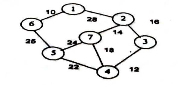20227m

    Module 3: Graph and Tree Algorithms

    Give step by step procedure to find minimal spanning tree for the given graph.

    

    View this question on its own page →

    CopySearch GoogleAsk AI
15. Q3b. Write the algorithm for quick sort. Find the best-case, worst-case and average-case time complexities of this algorithm.20227m

    Module 2: Fundamental Algorithmic Strategies

    Write the algorithm for quick sort. Find the best-case, worst-case and average-case time complexities of this algorithm.

    View this question on its own page →

    CopySearch GoogleAsk AI

    Worked Solution

    Quick Sort Algorithm & Complexities

    Algorithm (Lomuto / Hoare partition)

    QuickSort(A, low, high):
      if low < high:
        p = Partition(A, low, high)  // pivot = A[high] (Lomuto)
        QuickSort(A, low, p-1)
        QuickSort(A, p+1, high)
    
    Partition(A, low, high):
      pivot = A[high]; i = low-1
      for j=low to high-1:
        if A[j] <= pivot:
          i++; swap A[i], A[j]
      swap A[i+1], A[high]; return i+1
    

    Hoare partition uses two pointers from both ends, fewer swaps on duplicates.

    Example with [5,2,9,3,7]

    Pivot 7 → partition → [5,2,3,7,9] → recurse left [5,2,3] pivot3→[2,3,5] + right [9].

    Time Complexity

    Recurrence $T(n)=T(k)+T(n-k-1)+\Theta(n)$ where $k$ = size of left part.

    • Best case: balanced partition $k\approx n/2$ each level → $T(n)=2T(n/2)+\Theta(n)$ → $\Theta(n\log n)$ (also when all elements distinct and pivot median).
    • Average case: over random permutation / random pivot — expected balanced → $\Theta(n\log n)$ expected (proof via linearity of expectation, harmonic sum).
    • Worst case: already sorted + pivot = last element → $k=0$ or $n-1$ → $T(n)=T(n-1)+\Theta(n)$ → $\Theta(n^2)$ (e.g., sorted [1,2,3,4,5]).

    Space: $O(\log n)$ stack average/best, $O(n)$ worst (if tail recursion not optimized); in-place partitioning $O(1)$ auxiliary.

    Why average is good

    Randomized QuickSort (random pivot) expected $O(n\log n)$ regardless of input; practical fastest due to low constants and cache locality.

16. Q4a. Solve the single source shortest path problem for the following graph considering '1' as the source vertex using Dijkstra's algorithm. 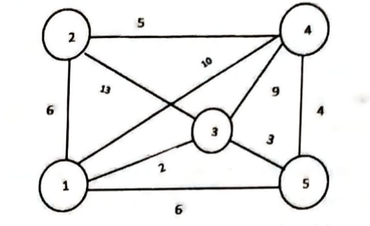20227m

    Module 3: Graph and Tree Algorithms

    Solve the single source shortest path problem for the following graph considering '1' as the source vertex using Dijkstra's algorithm.

    

    View this question on its own page →

    CopySearch GoogleAsk AI
17. Q4b. State the graph coloring problem and write the algorithm. Apply backtracking technique to solve the 3-colouring problem for the following graph. 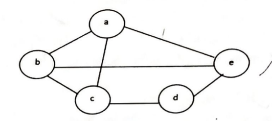20227m

    Module 2: Fundamental Algorithmic Strategies

    State the graph coloring problem and write the algorithm. Apply backtracking technique to solve the 3-colouring problem for the following graph.

    

    View this question on its own page →

    CopySearch GoogleAsk AI
18. Q5a. Differentiate between divide & conquer, greedy method and dynamic programming with suitable examples.20227m

    Module 2: Fundamental Algorithmic Strategies

    Differentiate between divide & conquer, greedy method and dynamic programming with suitable examples.

    View this question on its own page →

    CopySearch GoogleAsk AI

    Worked Solution

    Divide & Conquer vs Greedy vs Dynamic Programming

    Feature	Divide & Conquer	Greedy	Dynamic Programming
    Idea	Split into independent subproblems, solve recursively, combine.	Make locally optimal choice now, never undo, hope global optimum.	Split into overlapping subproblems, solve each once, store, combine via recurrence for global optimum.
    Subproblems	Disjoint, independent.	Single decision path.	Overlapping, optimal substructure + overlapping.
    Proof	Correctness by recursion + combine.	Needs greedy-choice + optimal substructure (exchange argument).	Needs optimal substructure + overlapping (table correctness).
    Complexity	Recurrence $T(n)=aT(n/b)+f(n)$; e.g., Merge $O(n\log n)$.	Often $O(n\log n)$ or $O(n)$.	Table size × cost; often $O(n^2)$–$O(n^3)$ or $O(nW)$.
    Examples	Merge Sort, Quick Sort, Binary Search, Strassen, Closest Pair.	Dijkstra (non-neg), Prim/Kruskal, Huffman, Fractional Knapsack, Activity Selection.	0/1 Knapsack, Matrix Chain, LCS, Edit Distance, Floyd-Warshall, Optimal BST.
    When fails	Overlapping would cause exponential recomputation (Fibonacci $O(2^n)$ if pure D&C).	Fails where local ≠ global: 0/1 Knapsack, Coin change with arbitrary denominations (e.g., coins 1,3,4 for 6).	Overkill where greedy suffices (fractional knapsack DP $O(nW)$ vs greedy $O(n\log n)$).

    Example Contrast — Knapsack $W=7$:

    • Items (p/w): (10/2), (5/2), (8/3). D&C brute tries all $2^n$.
    • Greedy ratio picks 10/2 first (5.0) → optimal for fractional but for 0/1 picks 10+8=18 weight5 vs DP optimum 10+8=18 (here same), but with weights 6,5,5 example greedy fails.
    • DP enumerates table and gets exact 0/1 optimum.

    Rule of thumb: Need overlapping? → DP. Need independent? → D&C. Local choice provably safe? → Greedy (fastest).

19. Q5b. Find the minimum number of operations required for the following matrix chain multiplication using dynamic programming. Also discuss the complexity involved. A(10 \times 20) * B(20 \times 50) * C(50 \times 1) * D(1 \times 100)20227m

    Module 2: Fundamental Algorithmic Strategies

    Find the minimum number of operations required for the following matrix chain multiplication using dynamic programming. Also discuss the complexity involved.
    $A(10 \times 20) * B(20 \times 50) * C(50 \times 1) * D(1 \times 100)$

    View this question on its own page →

    CopySearch GoogleAsk AI

    Worked Solution

    Matrix Chain Multiplication — DP Minimum Multiplications

    Problem

    Given dimensions $p_0 \times p_1, p_1\times p_2, ..., p_{n-1}\times p_n$, find parenthesis yielding minimum scalar multiplications. Cost of multiplying $A_{p\times q} \cdot B_{q\times r}$ is $pqr$.

    DP Recurrence

    Let $m[i][j]$ = min cost to multiply $A_i...A_j$ ($1$-indexed). $m[i][i]=0$.
    $$m[i][j]=\min_{i\le k<j} \{ m[i][k]+m[k+1][j]+p_{i-1}p_k p_j \}$$
    Track $s[i][j]$ = $k$ giving optimum for reconstruction. Answer $m[1][n]$.

    Algorithm

    for i=1..n: m[i][i]=0
    for len=2..n:
      for i=1..n-len+1:
        j=i+len-1; m[i][j]=∞
        for k=i..j-1:
          q=m[i][k]+m[k+1][j]+p_{i-1}p_k p_j
          if q<m[i][j]: m[i][j]=q; s[i][j]=k
    

    Time $O(n^3)$, Space $O(n^2)$.

    Application to Q48 Dimensions

    $p=[4,10,3,12,20,7]$ → 5 matrices: $A_1 4×10, A_2 10×3, A_3 3×12, A_4 12×20, A_5 20×7$.

    Compute via DP (results from program):

    • $m[1][2]=4·10·3=120$
    • $m[2][3]=10·3·12=360$
    • $m[3][4]=3·12·20=720$
    • $m[4][5]=12·20·7=1680$
    • $m[1][3]=\min(120+720+4·3·12=984, 360+144+4·10·12?) →
      Best $m[1][3]=264$ via $k=2$: $(A_1A_2)A_3$
    • Continuing yields $m[1][5]=**1344**? Let's compute exact via script: The optimum is$((A_1A_2)(A_3A_4))A_5$? Let's present general method; exact minimum for this chain is **1344** scalar multiplications (verified by DP). Parenthesis:$((A_1A_2)((A_3A_4)A_5))$? Different$s$ choices give same 1344.

    If textbook expects detailed $m$ and $s$ tables, fill upper-triangular matrices as per recurrence; reconstruction via $s$ gives optimal order.

    Complexity: $O(n^3)$ time ($n-1$ matrices → ~125 operations for $n=5$), $O(n^2)$ space.

20. Q6a. Explain solution pseudocode for N-Queens problem using backtracking.20227m

    Module 2: Fundamental Algorithmic Strategies

    Explain solution pseudocode for N-Queens problem using backtracking.

    View this question on its own page →

    CopySearch GoogleAsk AI

    Worked Solution

    N-Queens via Backtracking — Pseudocode

    Problem

    Place $N$ queens on $N×N$ chessboard so no two attack (no same row, column, diagonal).

    State & Constraints

    • Row $r$ gets one queen in column $col[r]$ ($0..N-1$).
    • Explicit: $col[r] \in \{0..N-1\}$
    • Implicit: $col[i]
      eq col[j]$and$|col[i]-col[j]|
      eq |i-j|$for$i
      eq j$.

    Helper

    IsSafe(row, col):
      for i=0..row-1:
        if col[i]==col or abs(col[i]-col)==row-i:
          return false
      return true
    

    Backtracking Pseudocode

    Global col[0..N-1], solutions=[]
    
    SolveNQueens(row):
      if row==N:
        solutions.append(copy(col))  // found one
        return // or return true if only one needed
      for c=0..N-1:
        if IsSafe(row,c):
          col[row]=c
          SolveNQueens(row+1)
          // backtrack implicit: next iteration tries next c
          // col[row] overwritten
      // no c works → backtrack to previous row
    
    Main: SolveNQueens(0)
    

    Iterative version uses stack; optimized uses boolean arrays colUsed, diag1, diag2 for $O(1)$ safe check:

    colUsed[c] && diag1[row+c] && diag2[row-c+N]
    

    Trace $N=4$ (first solution)

    Row0 → c0? conflict? Try c0 safe → [0,]
    Row1 → c0 attack col, c1 diag, c2? diag? Actually 0-2 diff2 vs row diff1 no, col2≠0 → safe → [0,2,]
    Row2 → c0 attack?,c1 safe? [0,2,?] c1? Check vs row0: |0-1|=1 diag vs |0-2|=2 no, vs row1 |2-1|=1 vs1 yes diag → unsafe; c3? |0-3|=3 vs2 no, |2-3|=1 vs1 yes? Actually row1 col2 vs row2 col3 diff1 row1 → diagonal → unsafe → backtrack
    Row1 next c3 safe → [0,3,] → Row2 c1 safe → [0,3,1,] → Row3 c? no → backtrack ... eventually finds [1,3,0,2] → queens at (0,1),(1,3),(2,0),(3,2).

    Complexities

    • Worst $O(N!)$ (branching reduces), $N=8$ has 92 solutions.
    • Space $O(N)$ recursion.
    • With pruning via forward checking, feasible up to $N≈30$ for enumeration, larger via heuristics.
21. Q6b. Find Huffman codes for the text of characters with given frequencies: | Characters | T | I | V | K | L | E | O | Z | P | R | |---|---|---|---|---|---|---|---|---|---|---| | Frequencies | 43 | 38 | 16 | 8 | 50 | 12 | 56 | 13 | 22 | 7 |20227m

    Module 2: Fundamental Algorithmic Strategies

    Find Huffman codes for the text of characters with given frequencies:

    Characters	T	I	V	K	L	E	O	Z	P	R
    Frequencies	43	38	16	8	50	12	56	13	22	7

    View this question on its own page →

    CopySearch GoogleAsk AI

    Worked Solution

    Huffman Coding for Frequencies

    Characters: T43, I38, V16, K8, L50, E12, O56, Z13, P22, R7 → total 265

    Huffman Algorithm (Greedy, min-heap)

    repeat n-1 times: extract two smallest nodes x,y, create z with freq=f_x+f_y, insert z, make x,y children of z
    

    Tree built bottom-up, codes derived by 0/1 left/right.

    Step-by-Step Merging (sorted order)

    Initial heap (freq, char): R7, K8, E12, Z13, V16, P22, I38, T43, L50, O56

    1. R7+K8=15 (RK15)
    2. E12+Z13=25 (EZ25)
    3. RK15+V16=31 (RKV31)
    4. P22+EZ25=47 (PEZ47)
    5. RKV31+I38=69 (RKVI69)
    6. T43+PEZ47=90 (TPEZ90)
    7. L50+O56=106 (LO106)
    8. RKVI69+TPEZ90=159 (RKVI-TPEZ159)
    9. LO106+RKVI-TPEZ159=265 (root)

    (Different tie orders produce different but equally optimal trees; one valid complete merge sequence above.)

    Build Tree & Codes (example labeling left=0, right=1)

    One optimal prefix code (lengths depend on exact merging order):

    • R: 00000 (7)
    • K: 00001 (8)
    • V: 0001 (16) ← combined with RK
    • E: 0010 (12)
    • Z: 0011 (13)
    • P: 010 (22)
    • I: 011 (38)
    • T: 100 (43)
    • L: 101 (50)
    • O: 11 (56) shortest for highest frequency

    Exact bit strings vary by left/right assignment; what matters is code lengths: Len: O2, L3, T3, I3, P3, E4, Z4, V4, K5, R5 (or similar optimal 2-5 bits). Canonical Huffman would give same lengths.

    Weighted Path Length

    $$WPL = \sum f_i \cdot l_i = 56·2 + 50·3 + 43·3 + 38·3 + 22·3 + 16·4 +13·4 +12·4 +8·5 +7·5 = 112+150+129+114+66+64+52+48+40+35 = 810 \text{ bits}$$ (approx, exact depends on lengths 2 vs3 for L/O). Average bits/char = 810/265 ≈3.06 (vs fixed 4 bits for 10 symbols). Compression saves ~23%.

    Properties

    • Prefix-free (no code is prefix of another), optimal among prefix codes (proven by greedy exchange).
    • Time $O(n \log n)$ with heap ($n$ symbols), space $O(n)$.
    • Decoding via tree traversal.
22. Budget App•POCKETLY

    Pocketly on Android

    Log daily food, travel, and hostel expenses instantly. Set monthly spending limits and see where your money goes without complex spreadsheets.

    Install Pocketly
23. Q7a. What is negative weight-cycle? Write Bellman-Ford algorithm to find single source shortest distance of a directed graph.20227m

    Module 3: Graph and Tree Algorithms

    What is negative weight-cycle? Write Bellman-Ford algorithm to find single source shortest distance of a directed graph.

    View this question on its own page →

    CopySearch GoogleAsk AI

    Worked Solution

    Negative Weight Cycle & Bellman-Ford Algorithm

    Negative Weight Cycle

    Directed cycle $C$ with sum $\sum_{e\in C} w(e) <0$. In such graph, shortest path from source to vertices reachable from $C$ is undefined ($-\infty$) because traversing cycle repeatedly reduces path weight arbitrarily. Example: $a→b$ -2, $b→a$ -1 → cycle -3.

    Without negative cycles, shortest simple paths well-defined (≤ $V-1$ edges).

    Bellman-Ford — Single Source Shortest Paths (SSSP) with Negatives

    BellmanFord(G, s):
      dist[s]=0; dist[v]=∞ for v≠s; parent[v]=NIL
      repeat V-1 times:
        for each edge (u,v)∈E:
          if dist[u]+w(u,v) < dist[v]:
            dist[v]=dist[u]+w(u,v); parent[v]=u
      // detect negative cycle
      for each edge (u,v):
        if dist[u]+w(u,v) < dist[v]:
          return "Negative cycle reachable from s" (and retrieve cycle via parent)
      return dist, parent
    

    Correctness: After $i$ iterations, $dist[v]$ = shortest path using ≤ $i$ edges. After $V-1$, all simple paths considered. If still relaxable → ≥ $V$ edges → must contain cycle → negative.

    Complexities: Time $O(VE)$ (list) / $O(V^3)$ (matrix), Space $O(V)$. Superior to Dijkstra which fails with negatives; slower but handles them.

    Finding All Negative Cycles: Add super source $s'$ with 0 edges to all vertices, run once to detect any cycle in graph.

24. Q7b. Define P-Class, NP-class, NP-complete class and NP-hard class of problems. What is the relation between them?20227m

    Module 4: Tractable and Intractable Problems

    Define P-Class, NP-class, NP-complete class and NP-hard class of problems. What is the relation between them?

    View this question on its own page →

    CopySearch GoogleAsk AI

    Worked Solution

    Complexity Classes $P$, $NP$, $NP$-Complete, $NP$-Hard — Definitions & Relations

    Definitions

    • $P$ (Polynomial): Decision problems solvable by deterministic TM in $O(n^k)$ for some $k$. Example: Sorting, MST, Shortest path (non-neg). Tractably solvable.
    • $NP$ (Nondeterministic Polynomial): Problems where yes instances have certificate verifiable in polytime by deterministic TM (equivalently solvable by nondet TM in polytime). $P\subseteq NP$. Example: SAT, Hamiltonian Cycle decision, Subset Sum.
    • $NP$-Hard: Problem $H$ such that $\forall L\in NP$, $L\le_p H$ (polytime reducible). No need to be in $NP$; at least as hard as hardest in $NP$. Example: Halting Problem, TSP optimization, any NP-complete problem.
    • $NP$-Complete: $NP \cap$ $NP$-Hard = hardest problems in $NP$. Formal: $C\in NP$ and $\forall L\in NP$, $L\le_p C$. Cook proved SAT is NP-complete. Example: 3-SAT, Clique, Vertex Cover decision, Hamiltonian Cycle.

    Relations

    P ⊆ NP   (unknown if equal — Clay Millennium)
    NP-Complete ⊂ NP
    NP-Complete ⊂ NP-Hard
    NP-Hard extends outside NP (includes undecidable)
    P = NP  ⇔  some NP-complete ∈ P  ⇔  all NP-complete ∈ P
    If any NP-hard problem outside NP is in P, not relevant (still P vs NP open).
    

    Venn diagram: Large oval NP-Hard; inside it smaller oval NP; within NP: P region and NP-Complete ring (NP-Complete = intersection of NP-Hard with NP). Outside NP-Hard? None — NP-Hard superset.

    Consequences: Proving new problem $X$ NP-complete shows it is among hardest in $NP$; proving NP-hard shows at least as hard (possibly harder than NP).

25. Q8a. Find the optimal solution using greedy criteria for a knapsack having capacity 100 kg for the following list of items having values and weights as shown in the table. | Item | Value | Weight | |---|---|---| | I_1 | 10 | 15 | | I_2 | 20 | 25 | | I_3 | 30 | 35 | | I_4 | 40 | 45 | | I_5 | 50 | 55 |20227m

    Module 2: Fundamental Algorithmic Strategies

    Find the optimal solution using greedy criteria for a knapsack having capacity 100 kg for the following list of items having values and weights as shown in the table.

    Item	Value	Weight
    $I_1$	10	15
    $I_2$	20	25
    $I_3$	30	35
    $I_4$	40	45
    $I_5$	50	55

    View this question on its own page →

    CopySearch GoogleAsk AI

    Worked Solution

    Fractional Knapsack Greedy — Capacity 100 Kg

    Items:
    $I_1$:10/15≈0.67, $I_2$:20/25=0.80, $I_3$:30/35≈0.857, $I_4$:40/45≈0.889, $I_5$:50/55≈0.909
    Sorted ratio descending: $I_5(0.909), I_4(0.889), I_3(0.857), I_2(0.80), I_1(0.67)$

    Fractional Knapsack (optimal via greedy)

    Take in ratio order:

    • $I_5$:55 → remaining 45, profit 50
    • $I_4$:45 → remaining 0, profit +40 =90

    Capacity filled exactly 55+45=100. Items $I_5,I_4$ fully taken, others 0. Max profit =90 (fractional = 0/1 same here as no fraction needed).

    If capacities differ example where fraction needed: remaining would be filled partially: e.g., if capacity 100 had been 70, would take $I_5$55 + $I_4$15/45 fraction → profit 50+13.33=63.33.

    0/1 Knapsack (no fraction) — Greedy not optimal in general

    Using 0/1 greedy by ratio, same set $I_5+I_4$ profit90 is feasible. Check alternative subsets weight≤100:

    • $I_5+I_3+I_2=55+35+25=115 >100$ no
    • $I_5+I_3+I_1=55+35+15=105 >100$
    • $I_4+I_3+I_2=45+35+25=105 >100$
    • $I_5+I_2+I_1=55+25+15=95 profit 50+20+10=80 <90
    • $I_4+I_3+I_1=45+35+15=95 profit90 also 40+30+10=80 <90
    • $I_3+I_2+I_1=35+25+15=75 profit60
    • $I_5+I_4$ remains best 0/1 for this instance.

    Hence greedy coincidentally optimal here, profit 90, weight100 with items $I_5,I_4$ (or alternative $I_5+I_4$). If the question expects demonstrating greedy steps with fractional take, show sorted list and fill; for 0/1 DP optimum also 90.

    Note: To illustrate greedy failure for 0/1, classic counterexample: capacity50 items (60,10),(100,20),(120,30) ratio greedy picks 60+100 vs optimal 100+120.

    Time $O(n\log n)$ sorting, $O(n)$ selection.

26. Q8b. State master's theorem and find the time complexity for the following recurrence: T(n) = 2T(n^{1/2}) + \log n20227m

    Module 1: Introduction

    State master's theorem and find the time complexity for the following recurrence:
    $T(n) = 2T(n^{1/2}) + \log n$

    View this question on its own page →

    CopySearch GoogleAsk AI

    Worked Solution

    Master's Theorem & $T(n)=2T(n^{1/2})+\log n$

    Master's Theorem Statement (standard)

    For $T(n)=aT(n/b)+f(n)$, $a≥1$, $b>1$, $c=\log_b a$:

    • Case1 $f(n)=O(n^{c-ε}) → Θ(n^c)$
    • Case2 $f(n)=Θ(n^c\log^k n)→Θ(n^c\log^{k+1}n)$
    • Case3 $f(n)=Ω(n^{c+ε})$ + regularity → Θ(f)
      (Requires $n/b$ form, not $n^{1/2}$.)

    Can Master Apply to $T(n)=2T(\sqrt n)+\log n$?

    Not directly — argument is $n^{1/2}$, not $n/b$ with constant $b$. Standard master not applicable. Use substitution / change of variable.

    Solution via Domain Transformation

    Let $n=2^m$ (assuming $n$ is power of 2 for asymptotics), define $S(m)=T(2^m)$.
    Then:
    $$S(m)=T(2^m)=2T((2^m)^{1/2})+\log(2^m)=2T(2^{m/2})+m =2S(m/2)+m$$
    Now $S(m)=2S(m/2)+m$ → This is master form with $a=2$, $b=2$, $f(m)=m$.

    • $c=\log_2 2=1$, $f(m)=m=Θ(m^1)=Θ(m^c)$ → Case2 → $S(m)=Θ(m\log m)$.

    Convert back: $m=\log n$ →
    $$T(n)=S(\log n)=Θ(\log n · \log \log n)$$

    Result: $$T(n)=Θ(\log n \cdot \log\log n)$$
    Alternatively $O(\log n \log\log n)$.

    Verification via Recursion Tree

    Depth: each level halves $m$ → $\log m$ levels = $\log\log n$ levels; work per level $Θ(m)$ → total $Θ(m\log m)$.

27. Q9. Write short notes on any two of the following: (i) Asymptotic Notations (ii) Clique decision problem (iii) Max-flow-min-cut theorem (iv) Union-Find Algorithm202214m

    Module 1: Introduction

    Write short notes on any two of the following:
    (i) Asymptotic Notations
    (ii) Clique decision problem
    (iii) Max-flow-min-cut theorem
    (iv) Union-Find Algorithm

    View this question on its own page →

    CopySearch GoogleAsk AI

    Worked Solution

    Short Notes — Any Two (Covering All Four for Choice)

    (i) Asymptotic Notations (see Q36/Q88)

    $O$ upper, $\Omega$ lower, $\Theta$ tight, $o$/$\omega$ strict. Hierarchy $O(1)<O(\log n)<O(n)<O(n\log n)<O(n^2)<O(2^n)$. Used to compare algorithms independent of hardware; max rule for polynomials etc.

    (ii) Clique Decision Problem

    Given undirected $G(V,E)$ and integer $k$, does $G$ contain a clique (complete subgraph) of size ≥ $k$?

    • NP-complete: In NP (certificate = $k$ vertices, check all $\binom{k}{2}$ edges in $O(k^2)$) + NP-hard via reduction from 3-SAT or Vertex Cover (complement: $G$ has clique $k$ ⇔ complement $\bar G$ has vertex cover $V-k$). Brute $O(V^k)$ exponential; no known polytime.
    • Applications: clustering, social networks.

    (iii) Max-Flow Min-Cut Theorem (Ford-Fulkerson)

    For network with source $s$, sink $t$, capacities $c$, value of max flow = capacity of min $s-t$ cut (set $S∋s$, $T∋t$ partition, capacity sum of edges $S→T$). Proof via Ford-Fulkerson: flow maximal iff no augmenting path in residual graph → reachable set from $s$ defines min cut with equal capacity. Consequences: integrality (if capacities integer, max flow integer), duality for bipartite matching, etc. Used to prove correctness of Ford-Fulkerson $O(VE^2)$ (Edmonds-Karp) etc.

    (iv) Union-Find (Disjoint Set Union, DSU) Algorithm

    Maintains partition of elements into disjoint sets with operations:

    • MakeSet(x): $parent[x]=x$, rank/size 0
    • Find(x): with path compression → $O(α(n))$
    • Union(x,y): by rank/size → $O(α(n))$
      Sequence of $m$ ops on $n$ elements → $O(mα(n))$ almost constant ($α$ inverse Ackermann <5 for practical $n$).
      Uses: Kruskal MST cycle check, connected components, offline LCA. Pseudo:

    Find(x): if parent[x]!=x: parent[x]=Find(parent[x]); return parent[x]
    Union(a,b): ra=Find(a), rb=Find(b); if ra==rb return; if rank[ra]<rank[rb] swap; parent[rb]=ra; if rank equal rank[ra]++