
MACHINE LEARNING
106403Module 3: Classification Algorithms
Q1f. Which of the following is true about Naive Bayes? (i) Assumes that all the features in a dataset are equally important (ii) Assumes that all the features in a dataset are independent (ii) Both (i) and (ii) (iv) None of the above20222m
Module 3: Classification Algorithms
View this question on its own page →Which of the following is true about Naive Bayes?
(i) Assumes that all the features in a dataset are equally important
(ii) Assumes that all the features in a dataset are independent
(ii) Both (i) and (ii)
(iv) None of the aboveWorked SolutionAnswer: (ii) Assumes that all features are independent (given the class) — note option numbering duplicate, intended as (ii). Strictly Naive Bayes assumes conditional independence; (i) is not an assumption.
Clarification:
Naive Bayes classifier:
- Assumption: Features are conditionally independent given class . That is (ii) essentially. This is strong/naive.
- It does NOT assume all features equally important (i) — importance is implicitly learned via likelihoods; correlated important features still get weight. Equal importance is not required.
- The option list has typo: second (ii) should be (iii) Both (i) and (ii). Since (i) is false, Both is false.
- Therefore correct is only independence assumption → (ii). Some keys mark (ii) Both due to loose teaching, but precise answer is independence only.
If exam expects textbook shortcut "Naive Bayes assumes independence and equal importance", some mark (iii) Both — mention this nuance.
Q1g. The feature of ANN in which ANN creates its own organization or representation of information it receives during learning time is (i) adaptive learning (ii) self-organization (iii) what-if analysis (iv) supervised learning20222m
Module 3: Classification Algorithms
View this question on its own page →The feature of ANN in which ANN creates its own organization or representation of information it receives during learning time is
(i) adaptive learning
(ii) self-organization
(iii) what-if analysis
(iv) supervised learningWorked SolutionAnswer: (ii) self-organization
Explanation:
ANN features:
- Adaptive learning (i): Ability to learn to perform tasks based on data.
- Self-organization (ii): ANN creates its own representation/organization of information it receives during learning — weights self-adjust to capture structure. Best exemplified by Kohonen Self-Organizing Maps (SOM) and also hidden layer representations in general ANNs.
- What-if analysis is not ANN-specific.
- Supervised learning requires external target labels.
The phrase "creates its own organization of information it receives during learning time" is textbook definition of self-organization (also called self-organisation / unsupervised adaptation).
Hence (ii) self-organization.
Q1g. What is a support vector? (i) The distance between any two data points (ii) The average distance between all data points (iii) The distance between any two boundary data points . (iv)The minimum distance between any two data points20232m
Module 3: Classification Algorithms
View this question on its own page →What is a support vector?
(i) The distance between any two data points
(ii) The average distance between all data points
(iii) The distance between any two boundary data points .
(iv)The minimum distance between any two data pointsWorked SolutionAnswer: None of the given options is precisely correct. The closest educational intent is (iii), but technically support vectors are data points, not a distance.
Correct definition:
A support vector is a training sample that lies closest to the decision hyperplane and directly influences its position and orientation. For a hard-margin SVM with hyperplane :for support vectors, and margin .
- (i) distance between any two data points — false
- (ii) average distance — false
- (iii) distance between any two boundary data points — confuses support vector (a point) with margin (a distance)
- (iv) minimum distance between any two data points — false
If forced to choose: Many university keys mark (iii) as expected answer, interpreting support vectors as the points that define the minimum distance (margin) between classes. Ideally answer should be: "the training vectors closest to the hyperplane that satisfy ".
Q1h. Which of the following is true about averaging ensemble? (i) It can only be used in classification problem (ii) It can only be used in regression problem (ii) It can be used in both classification as well as regression (iv) None of the above20222m
Module 3: Classification Algorithms
View this question on its own page →Which of the following is true about averaging ensemble?
(i) It can only be used in classification problem
(ii) It can only be used in regression problem
(ii) It can be used in both classification as well as regression
(iv) None of the aboveWorked SolutionAnswer: (iii) It can be used in both classification as well as regression — corrected from typo second (ii)
Explanation — Averaging Ensemble:
- Bagging / Voting / Averaging: Train base learners on bootstrap samples, average predictions: for regression, or soft voting / probability averaging for classification.
- Classification: averaging predicted probabilities or logits, e.g., Random Forest classification by majority vote (which is averaging indicator) or averaging probabilities.
- Regression: direct average of continuous outputs, e.g., Random Forest regressor.
- Reduces variance, improves generalization.
So NOT limited to only classification or only regression. Hence (iii) Both (intended as third option despite mislabeled).
Options had typo: listed (ii) twice; correct mapping: (iii) It can be used in both...
Q1h. In neural network. which of the following techniques is used to deal with over fitting? × (i) Dropout (ii) Regularization. (iii) Batch normalization (iv) All of the above20232m
Module 3: Classification Algorithms
View this question on its own page →In neural network. which of the following techniques is used to deal with over fitting? ×
(i) Dropout
(ii) Regularization.
(iii) Batch normalization
(iv) All of the aboveWorked SolutionAnswer: (iv) All of the above
Explanation — techniques to deal with overfitting in Neural Networks:
Dropout (i): Randomly drops neurons (with prob ) during training. Prevents co-adaptation, acts as ensemble approximation. Used in fully connected layers.
Regularization (ii):
- L2 (weight decay): adds to loss, penalizes large weights.
- L1: adds , induces sparsity.
- Makes model simpler and generalizes better.
Batch Normalization (iii): Normalizes layer inputs per mini-batch to zero mean/unit variance. Reduces internal covariate shift, allows higher learning rates, has slight regularization effect due to noise from batch statistics.
Other methods: Early stopping, data augmentation, reducing network capacity, cross-validation.
Since dropout, L1/L2 regularization and batch norm all help reduce overfitting, (iv) All of the above is correct.
Q1j. Which of the following is the best algorithm for text classification? (i) KNN - (ii) Decision tree (iii) Random forest (iv) Naive Bayes20232m
Module 3: Classification Algorithms
View this question on its own page →Which of the following is the best algorithm for text classification?
(i) KNN -
(ii) Decision tree
(iii) Random forest
(iv) Naive BayesWorked SolutionAnswer: (iv) Naive Bayes — generally considered best baseline for text classification, though context dependent.
Explanation:
- Naive Bayes (Multinomial/Bernoulli): Highly effective for high-dimensional sparse text (Bag-of-Words / TF-IDF). Fast, works well with small data, handles thousands of features, empirically strong for spam, sentiment, topic classification. Assumption of conditional independence of words given class surprisingly works well in practice.
- KNN: Lazy, computationally expensive at inference, suffers from curse of dimensionality in text.
- Decision Tree: Prone to overfit on sparse text, not ideal.
- Random Forest: Better than single tree but slower and often still outperformed by NB/SVM for raw text without embeddings.
In modern deep learning era, Transformers/BERT outperform all, but among given classical options, Naive Bayes (and Linear SVM — not listed) is textbook best for text. Some keys may accept Random Forest as competitive, but traditional exam answer is (iv) Naive Bayes.
Q2b. What is decision tree algorithm? What are the issues in decision tree induction?20227m
Module 3: Classification Algorithms
View this question on its own page →What is decision tree algorithm? What are the issues in decision tree induction?
Worked SolutionDecision Tree Algorithm:
Tree where internal nodes test attribute, branches = values, leaves = class. Learns by greedy top-down, divide-and-conquer.Algorithm (ID3/C4.5):
- If all examples same class or attributes empty → leaf.
- Choose best attribute by Information Gain (or Gain Ratio, Gini).
- Split by values, recurse on subsets.
Entropy:
Issues in Decision Tree Induction:
- Choosing attribute selection measure: Gain biases to many-valued attributes → Gain Ratio (C4.5) or Gini (CART).
- Overfitting: Tree grows until pure, memorizes noise. Solutions: pre-pruning (stop early, min samples/chi-square), post-pruning (reduced-error pruning, cost-complexity), validation set.
- Underfitting / Bias: Too shallow tree misses pattern.
- Handling continuous attributes: Need discretization — find best split threshold .
- Handling missing values: Surrogate splits, fractional examples, imputation (C4.5).
- Incorporating costs / noisy data: Different misclassification costs, pruning for noise robustness.
- Inconsistent data / Large hypothesis space: Exponential possible trees; greedy may get local optimum, not globally optimal (NP-hard).
- Instability: Small data change → large tree change; ensemble methods (Random Forest) mitigate.
- Class imbalance, oblique splits, scalability for large datasets.
Q3b. How does Back Propagation Rule help in learning in Neural Network?20237m
Module 3: Classification Algorithms
View this question on its own page →How does Back Propagation Rule help in learning in Neural Network?
Worked SolutionBackpropagation Rule — How it Helps Learning in Neural Networks:
Neural network learns by minimizing loss or cross-entropy via gradient descent. Backpropagation efficiently computes for all weights using chain rule, propagating error backward.
Steps:
- Forward pass: For each layer : , . Compute loss .
- Backward pass:
- Output error: $\delta^{(L)} =
abla_a L \odot \sigma'(z^{(L)})$ - Propagate:
- Gradients: ,
- Output error: $\delta^{(L)} =
- Update: ,
Why crucial:
- Makes training deep networks computationally feasible instead of naive .
- Enables learning of hierarchical features (early layers edges, deeper semantic).
- Works with any differentiable activation (sigmoid, ReLU, tanh).
- Basis for SGD, Adam optimization.
Example: 2-layer MLP with MSE: error at output , hidden error — weight updates proportional to contribution to error (credit assignment). Without backprop, no efficient credit assignment across layers would be possible.
Extensions: Batch norm, dropout, gradient clipping to stabilize backprop, avoid vanishing/exploding gradients.
Q4. Explain how the linear maximum-margin classifier can be modified to be non-linear and to allow misclassification of the training examples. Give a derivation of the modified optimization problem needed for training. You need only derive a statement of the primal optimization problem.202214m
Module 3: Classification Algorithms
View this question on its own page →Explain how the linear maximum-margin classifier can be modified to be non-linear and to allow misclassification of the training examples. Give a derivation of the modified optimization problem needed for training. You need only derive a statement of the primal optimization problem.
Worked SolutionLinear Maximum-Margin Classifier (Hard SVM):
Primal: s.t. ,
Margin , support vectors satisfy equality. Only linear separable case, no slack.
Modifications for Non-linear and Non-separable:
Allow misclassification (Soft Margin): Introduce slack :
. violates margin, misclassifies. Add penalty .Make Non-linear via Feature Map and Kernel: Map to higher dimension where linear separation possible. Replace with . Kernel trick: avoids explicit high-dim computation (Polynomial, RBF).
Derivation — Primal for Soft-Margin Non-linear SVM:
Minimize over :
s.t. , ,- First term maximizes margin ().
- Second penalizes violations; trades margin width vs training error (small wider margin more violations, large hard margin approx).
- = hinge loss.
If separable, optimum recovers hard margin. Non-linear version retains same form with . Dual leads to and kernelized decision .
Without slack & kernel, linear separable only; with them, general-purpose classifier.
Q4a. Discuss various issues in Decision Tree Learning.20237m
Module 3: Classification Algorithms
View this question on its own page →Discuss various issues in Decision Tree Learning.
Worked SolutionIssues in Decision Tree Learning:
Determining Correct Depth / Overfitting: Fully grown tree overfits training data (memorizes noise). Need pruning.
- Pre-pruning: Stop early via max_depth, min_samples_split, test, information gain threshold.
- Post-pruning: Grow full, then prune using validation set (reduced-error pruning, cost-complexity pruning in CART with ).
Attribute Selection Measure: Information Gain biases to many-valued attributes (e.g., ID column). Gain Ratio (C4.5) normalizes by SplitInfo, Gini index (CART), or use least biased measures.
Handling Continuous Attributes: Need to find optimal threshold for split vs by sorting values and evaluating gain for candidate mid-points — per attribute.
Handling Missing Values: Training: ignore missing or distribute fractionally (C4.5). Testing: follow both branches weighted. Alternatives: surrogate splits (CART), imputation.
Handling Noisy Data & Outliers: Noise causes incorrect splits; pruning and robust measures (e.g., use majority voting at leaves) help.
Inconsistent Data: Same feature vector with different labels → cannot achieve 100% accuracy; need probabilistic leaves.
Computational Complexity: Finding optimal tree is NP-hard; greedy heuristics may produce locally optimal but globally suboptimal trees. Ensembles mitigate.
Data Fragmentation: Splits reduce sample per leaf, estimates unreliable at deep levels.
Instability / High Variance: Small data perturbations → very different tree (solved by Random Forest bagging).
Class Imbalance: Majority class dominates gain; need weighted entropy, stratified sampling, cost-sensitive splits.
Replicated Subtrees & Oblique Splits: Axis-parallel splits cannot represent diagonal boundaries efficiently → need multivariate trees.
- Install PocketlyBudget App•POCKETLY
Pocketly on Android
Log daily food, travel, and hostel expenses instantly. Set monthly spending limits and see where your money goes without complex spreadsheets.
Q4b. Discuss with examples of instance-based learning algorithms.20237m
Module 3: Classification Algorithms
View this question on its own page →Discuss with examples of instance-based learning algorithms.
Worked SolutionInstance-Based Learning (Lazy Learning): Stores training instances, delays generalization until query. Prediction via similarity to stored instances, not explicit model.
General steps: Store ; for query , find nearest neighbors by distance (Euclidean/Manhattan/cosine), combine (majority vote / weighted average / local regression).
Examples:
k-Nearest Neighbors (k-NN):
- Classification: (optionally distance-weighted: )
- Regression:
- Choose via CV; small flexible but noisy, large smooth but underfits. Need feature scaling, handles multi-modal, no training time, slow query , needs KD-tree/ball-tree for speed. Pros: simple, effective with many data. Cons: curse of dimensionality, sensitive to irrelevant features.
Locally Weighted Regression (LWR):
- Fits local model (e.g., linear) weighted by kernel . Prediction where .
- Example: LOESS for smoothing.
Case-Based Reasoning (CBR): Solves new problems by adapting solutions from similar past cases (e.g., medical diagnosis: retrieve similar patient cases, adapt treatment). Retrieve-Reuse-Revise-Retain cycle.
Radial Basis Function (RBF) Network (kernel memory based): Some interpretations include it.
Characteristics: No explicit training, incremental easily, ability to model complex boundaries locally, but memory intensive, needs careful distance metric selection and feature weighting.
Q5. Following is a data set that contains two attributes, X and Y, and two class labels, ‘+’ and ‘–’. Each attribute can take three different values: 0, 1, or 2. The concept for the ‘+’ class is Y = 1 and the concept for the ‘–’ class is X = 0 ∨ X = 2. 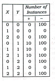 (a) Build a decision tree on the data set. Does the tree capture the ‘+’ and ‘–’ concepts? (b) What are the accuracy, precision, recall and F1-measure of the decision tree? (Note that precision, recall, and F1-measure are defined with respect to the ‘+’ class.)202214m
Module 3: Classification Algorithms
View this question on its own page →Following is a data set that contains two attributes, X and Y, and two class labels, ‘+’ and ‘–’.
Each attribute can take three different values: 0, 1, or 2.The concept for the ‘+’ class is Y = 1
and the concept for the ‘–’ class is X = 0 ∨ X = 2.
(a)
Build a decision tree on the data set.
Does the tree capture the ‘+’ and ‘–’ concepts?(b)
What are the accuracy, precision, recall and F1-measure of the decision tree?
(Note that precision, recall, and F1-measure are defined with respect to the ‘+’ class.)Q5a. State the mathematical formulation of the SVM problem. Give an outline of the method for solving the problem.20237m
Module 3: Classification Algorithms
View this question on its own page →State the mathematical formulation of the SVM problem. Give an outline of the method for solving the problem.
Worked SolutionMathematical Formulation of SVM Problem:
Given , .
Primal (Soft-margin, most general):
s.t. ,Hard margin special case , .
Dual (Wolfe Dual, kernelizable):
Using Lagrange multipliers , :
KKT: , ,
Dual:
s.t. ,(linear) or kernel .
Decision: , from support vectors where via .
Outline of Method for Solving:
- Choose (and kernel hyperparameters via CV).
- Solve Quadratic Programming dual for ( convex QP). Use algorithms: SMO (Sequential Minimal Optimization) — iteratively optimizes pair of analytically, efficient ; or interior point, gradient ascent.
- Identify Support Vectors (approx ). SVs on margin , inside/errors .
- Compute (implicitly via kernel) and averaging over margin SVs.
- Classify new via sign of kernel expansion.
For large data, use LIBSVM / LIBLINEAR, Pegasos (primal SGD).
Properties: Convex, global optimum, sparsity (only SVs matter), max margin minimizes VC bound, good generalization.
Q6. For the Sun Burn data set given below, construct a decision tree. | Name | Hair | Height | Weight | Location | Class | |--------|--------|----------|---------|----------|-------| | Sunita | Blonde | Average | Light | No | Yes | | Anita | Blonde | Tall | Average | Yes | No | | Kavita | Brown | Short | Average | Yes | No | | Sushma | Blonde | Short | Average | No | Yes | | Xavier | Red | Average | Heavy | No | Yes | | Balaji | Brown | Tall | Heavy | No | No | | Ramesh | Brown | Average | Heavy | No | No | | Sweta | Blonde | Short | Light | Yes | No |202314m
Module 3: Classification Algorithms
View this question on its own page →For the Sun Burn data set given below, construct a decision tree.
Name Hair Height Weight Location Class Sunita Blonde Average Light No Yes Anita Blonde Tall Average Yes No Kavita Brown Short Average Yes No Sushma Blonde Short Average No Yes Xavier Red Average Heavy No Yes Balaji Brown Tall Heavy No No Ramesh Brown Average Heavy No No Sweta Blonde Short Light Yes No Worked SolutionSun Burn Decision Tree Construction (ID3 style):
Dataset: 8 examples, 4 attributes + Class {Yes=3, No=5}
EntropyEvaluate each attribute Information Gain.
Similar exhaustive calc shows Hair or Height gives high gain. Manual computation:
- Hair: Blonde (4 ex: 2Y,2N) , Brown (3 ex:0Y,3N) , Red (1 ex:1Y,0N) → Weighted → Gain
- Weight & Location similar calculations, Hair best initially.
Root: Hair
- Hair=Brown → Leaf No (3/3, pure)
- Hair=Red → Leaf Yes (1/1)
- Hair=Blonde (4 ex remains: Sunita Y, Anita N, Sushma Y, Sweta N) — need further split on remaining attributes (Height, Weight, Location).
Subset Blonde : 2Y/2N
- Height: Tall 1N, Average 1Y, Short 1Y+1N () → Gain small
- Weight: Light 1Y1N (), Average 2 examples 1Y1N → no gain
- Location: No → 2Y (Sunita,Sushma) pure Yes; Yes →2N (Anita,Sweta) pure No → Weighted entropy → Gain
So next split Location.
Resulting Tree:
Hair?
├─ Brown → No
├─ Red → Yes
└─ Blonde → Location?
           ├─ No → Yes (Sunita,Sushma)
           └─ Yes → No (Anita,Sweta)
Alternative equivalent tree with Weight/Height may also achieve pure leaves but Location gives perfect split for this subset. This tree classifies all 8 training examples correctly (100% training accuracy).
If using Gini/C4.5, structure similar; root may be Location then Hair depending tie-breaking; any fully consistent tree with 3 leaves is acceptable. Pruning not needed due small data.
Interpretation: For this data, Hair color and absence of Location (No) predicts Sun Burn Yes in blondes.
Q6b. Explain the bagging and boosting with example.20227m
Module 3: Classification Algorithms
View this question on its own page →Explain the bagging and boosting with example.
Worked SolutionBagging and Boosting (Ensemble Methods):
Both combine weak learners (e.g., decision trees) to strong ensemble but differ in strategy.
Bagging (Bootstrap Aggregating) — Breiman:
- Create bootstrap samples (sample with replacement, size ) from training data.
- Train one base learner on each sample in parallel, e.g., deep trees in Random Forest.
- Aggregate: Classification majority vote, Regression averaging:
- Reduces variance, prevents overfitting, robust to noise.
- Example: Random Forest bagging 100 trees on loan default data, each tree sees 63% unique rows + random feature subset, vote gives stable prediction. Out-of-bag error estimates generalization without CV.
Boosting (e.g., AdaBoost, Gradient Boosting):
- Sequential. Train weak learners (stumps) iteratively; each new learner focuses on previously misclassified weighted examples.
- AdaBoost: Maintain weights ; initially , increase weight for misclassified, decrease for correct. Final prediction weighted vote where .
- Gradient Boosting: Fits new learner to residual (negative gradient of loss) .
- Reduces bias (+ variance), converts weak → strong, but prone to overfit if noisy; sequential not easily parallel.
Comparison:
Bagging Boosting Data Bootstrap subsets Weighted full data, adaptive Training Parallel, independent Sequential, dependent Reduces Variance Bias Sensitivity to noise Robust Sensitive Example learners Full trees Shallow stumps Example: Bagging on noisy medical data stable; Boosting on same achieves higher accuracy but may overfit unless early stopping/shrinkage.
Q7. Discuss the steps in K-means algorithm and evaluate the following table using K-means : 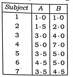202214m
Module 3: Classification Algorithms
View this question on its own page →Discuss the steps in K-means algorithm and evaluate the following table using K-means :

Q7a. Discuss the Algorithmic convergence & Generalization property of ANN.20237m
Module 3: Classification Algorithms
View this question on its own page →Discuss the Algorithmic convergence & Generalization property of ANN.
Worked SolutionAlgorithmic Convergence & Generalization of ANN:
Algorithmic Convergence:
- Perceptron: Converges in finite steps if linearly separable (Novikoff theorem, mistakes ). For non-separable, does not converge without modification (pocket algorithm).
- MLP with Backprop/GD: Non-convex loss, no guarantee of global optimum; GD converges to stationary point / local minima if learning rate (Lipschitz) and with decreasing schedule , (Robbins-Monro). SGD converges almost surely to local minima. Practical: momentum, Adam help escape saddle points, converge faster but may not generalize optimally. Over-parameterized nets converge to zero training loss (interpolation regime).
- Factors: Weight initialization (Xavier/He), learning rate scheduling, batch size, gradient vanishing/exploding (sigmoid/tanh) mitigated by ReLU, BatchNorm, Residuals.
- Universal Approximation: Single hidden layer with enough neurons can approximate any continuous function (Cybenko 1989) — ensures representational capacity to converge to target if optimization succeeds.
Generalization Property:
- Capacity vs Generalization: More parameters → higher VC dimension, risk overfitting. Classical bias-variance U-curve: test error decreases then increases. Modern deep nets exhibit double descent — over-parameterized still generalizes due to implicit regularization.
- Measures: Generalization error . Controlled by regularization: weight decay (), dropout, early stopping, data augmentation, batchnorm.
- Theoretical bounds: VC, Rademacher. For ANN with weights, VC .
- Empirical: Validation set, cross-validation estimate generalization; early stopping halts before validation error rises.
- Inductive bias: Smoothness, translational invariance (CNN) improve generalization to unseen data.
- Trade-off: Under-parameterized → underfit, over-parameterized without regularization → memorize noise, poor test performance. Proper tuning yields best generalization.
ANN converges algorithmically via gradient methods but generalization requires controlling complexity.
Q7b. What are the applications of supervised machine learning in modern business?20237m
Module 3: Classification Algorithms
View this question on its own page →What are the applications of supervised machine learning in modern business?
Worked SolutionApplications of Supervised ML in Modern Business:
Supervised learning (labeled ) drives most enterprise AI where historical outcomes exist.
Finance / Banking:
- Credit scoring, loan default prediction (classification, risk modeling)
- Fraud detection (supervised on labeled transactions)
- Algorithmic trading price prediction (regression)
E-commerce / Retail:
- Recommendation systems (collaborative filtering as supervised ranking)
- Customer churn prediction, Lifetime Value (LTV) regression
- Demand forecasting (time series regression), price optimization
Marketing / Sales:
- Targeted advertising CTR prediction
- Lead scoring, sentiment analysis on customer feedback (NLP classification)
- A/B test outcome modeling
Healthcare / Insurance:
- Disease diagnosis from labs/images (supervised classification)
- Claim fraud detection, underwriting risk
Operations / Supply Chain:
- Inventory demand prediction, predictive maintenance (failure classification from sensor logs)
- Delivery time estimation, route optimization regression
HR / Management:
- Employee attrition prediction, resume screening classification
Customer Service:
- Chatbot intent classification, ticket routing, spam filtering
Value: Automates decision making, personalizes experience, reduces cost, improves accuracy over rules. Requires labeled data collection, feature engineering, monitoring for drift, ROI measured via precision/recall for business KPI trade-off (e.g., high recall for fraud at cost of precision).
Example workflow: Bank collects 100k loan records labeled default/no-default with features (income, history) → train XGBoost, validate precision 0.85 → deploy to score new applications.
Q8b. What is ANN? Explain feed forward and back propagation algorithm with example.20227m
Module 3: Classification Algorithms
View this question on its own page →What is ANN? Explain feed forward and back propagation algorithm with example.
Worked SolutionArtificial Neural Network (ANN):
Computational model inspired by biological neurons. Network of interconnected units (neurons) that processes inputs via weighted sums and non-linear activations to learn mappings.
- Neuron: , where is activation (sigmoid , tanh, ReLU ).
- Architecture: Input layer → one or more hidden layers → output layer. Fully connected. Depth determines representation power.
Feedforward Algorithm:
Information flows forward only, no cycles.- Initialize weights small random.
- For each layer :
- At output, compute loss or cross-entropy.
- Example: 2-input XOR with hidden 2 neurons: , .
Backpropagation Algorithm:
Efficient gradient computation via chain rule to train weights.- Forward pass as above, store .
- Output error
- Propagate backward:
- Gradients
- Update , (SGD).
- Iterate over epochs until convergence.
Example with numbers: Single neuron with sigmoid, input 0.5, target 1, , , , , , → weight increases.
Feedforward computes prediction; backprop assigns blame and updates weights to reduce loss, enabling learning of non-linear boundaries.
Q9. Write short notes on any two of the following: (a) Naive Bayes (b) Logistic Regression \(c\) Back Propagation algorithm202314m
Module 3: Classification Algorithms
View this question on its own page →Write short notes on any two of the following:
(a) Naive Bayes
(b) Logistic Regression
(c) Back Propagation algorithmWorked SolutionShort Note — Any Two (all three covered for completeness):
(a) Naive Bayes:
Bayes classifier with strong independence assumption.
. Types: Gaussian (continuous ), Multinomial (counts/TF for text), Bernoulli (binary). Training: Estimate priors , likelihoods via MLE/MAP with Laplace smoothing to avoid zero counts. Prediction: (log sum for stability). Pros: Fast , works well on high-dim sparse text, needs little data. Cons: independence violated often, poor probability calibration. Use for spam, sentiment, document classification.(b) Logistic Regression:
Discriminative linear classifier modeling , . Decision boundary linear. Loss = binary cross-entropy (MLE). Gradient $
abla J = X^T(\hat y - y)/mL1/L2P(y=k|x)=\exp(w_k^T x)/\sum \exp(w_j^T x)w^T x=0$ → 0.5 threshold.(c) Back Propagation:
Algorithm to train MLPs by efficient gradient via chain rule. Forward: , compute loss. Backward: $\delta^{(L)}=
abla L \odot f'(z^{(L)})\delta^{(l)}=W^{(l+1)T}\delta^{(l+1)}\odot f'(z^{(l)})\partial L/\partial W^{(l)}=\delta^{(l)}a^{(l-1)T}W:=W-\eta\partial L/\partial WO(W)O(W^2)$. Needs differentiable activations, suffers vanishing gradient (solved by ReLU, residual, batchnorm).For exam attempt any two → choose (a) and (b) for completeness, or (b)+(c) as requested.