2022 question paper

MACHINE LEARNING

22 questions

1. Q1a. Which of the following is correct use of cross validation? (i) Selecting variables to include in a model (ii) Comparing predictors (iii) Electing parameters in prediction function (iv) All of the above20222m

   Module 1: Introduction

   Which of the following is correct use of cross validation?
   (i) Selecting variables to include in a model
   (ii) Comparing predictors
   (iii) Electing parameters in prediction function
   (iv) All of the above

   View this question on its own page →

   CopySearch GoogleAsk AI

   Worked Solution

   Answer: (iv) All of the above

   Correct uses of Cross Validation (CV):

   Cross validation (k-fold, LOOCV, stratified) estimates generalization performance by partitioning data into train/validation folds repeatedly.

   1. (i) Selecting variables / feature selection: CV error is used to compare subsets of features and choose set with lowest validation error, avoiding overfitting.
   2. (ii) Comparing predictors / model selection: Compare different model families (e.g., linear vs tree vs SVM) on CV score.
   3. (iii) Electing / selecting parameters in prediction function (hyperparameter tuning): e.g., choosing $k$ in KNN, $\lambda$ in ridge, $C$, $\gamma$ in SVM via grid search with CV. Also called hyperparameter optimization.

   Since all three are standard applications, (iv) All of the above is correct.

   Additional note: CV does not train final model; after selection, model is retrained on full training data and evaluated on held-out test set.

2. Q1b. Which of the following statement(s) is/are true for Gradient Decent (GD) and Stochastic Gradient Decent (SGD)? (1) In GD and SGD, you update a set of parameters in an iterative manner to function. minimize the error (2) In SGD, you have to run through all the samples in your training set for a single update of a parameter in each iteration. (3) In GD, you either use the entire data or a subset of training data to update a parameter in each iteration. (i) Only (1) (ii) (1) and (2) only (iii) (3) and (2) only (iv) (1), (2) and (3)20222m

   Module 1: Introduction

   Which of the following statement(s) is/are true for Gradient Decent (GD) and Stochastic Gradient Decent (SGD)?
   (1) In GD and SGD, you update a set of parameters in an iterative manner to function. minimize the error
   (2) In SGD, you have to run through all the samples in your training set for a single update of a parameter in each iteration.
   (3) In GD, you either use the entire data or a subset of training data to update a parameter in each iteration.

   (i) Only (1)
   (ii) (1) and (2) only
   (iii) (3) and (2) only
   (iv) (1), (2) and (3)

   View this question on its own page →

   CopySearch GoogleAsk AI

   Worked Solution

   Answer: (i) Only (1) — as per correct ML theory. Note many exam keys incorrectly mark (ii) due to typo; clarified below.

   Statement analysis:

   • (1) In GD and SGD, you update a set of parameters iteratively to minimize the error — TRUE. Both are iterative optimization algorithms: $w := w - \eta
     abla J(w)$.

   • (2) In SGD you have to run through all samples for a single update — FALSE. SGD uses one randomly chosen sample (or one mini-batch) per update. Statement describes Batch GD, not SGD. This is a common textbook error in the question.

   • (3) In GD you either use entire data or subset to update — FALSE. Standard GD uses entire training set per update. Using a subset is Mini-batch GD or SGD, not vanilla GD.

   Strictly: only (1) is true → (i) Only (1). If exam expects (ii) or (iii), it has swapped definitions. Conceptual correct behavior:

   • GD: one update per epoch using all $m$ examples — expensive but stable.
   • SGD: one update per example — noisy but fast, frequent updates.
   • Mini-batch: compromise (e.g., 32/64 samples).

3. Q1c. What makes the difference between good decisions and bad decisions? (i) A good decision is based on logic (ii) A good decision considers all available data (iii) A good decision considers all alternatives (iv) A good decision applies quantitative approaches20222m

   Module 2: Linear Models and Bayesian Learning

   What makes the difference between good decisions and bad decisions?
   (i) A good decision is based on logic
   (ii) A good decision considers all available data
   (iii) A good decision considers all alternatives
   (iv) A good decision applies quantitative approaches

   View this question on its own page →

   CopySearch GoogleAsk AI

   Worked Solution

   Answer: (iv) A good decision applies quantitative approaches — though in ML/decision theory all (i)-(iii) also contribute, expected exam answer is (iv).

   Explanation:

   In Statistical Decision Theory / ML:

   • Good decisions are not just based on logic (i) alone — logic without data is insufficient.
   • Considering all data (ii) and all alternatives (iii) are part of rational decision making, but alone not distinctive.
   • Quantitative approaches (iv) — using probability, expected loss/risk $R(a) = \int L(a,y) p(y|x) dy$, utility, optimization — differentiate good from bad decisions objectively. This aligns with Bayesian decision theory, where you choose action $a^* = \arg\min_a E[L]$.

   Textbook often phrases: "A good decision is based on logic, considers all available data and alternatives, and applies quantitative approaches." If single best is asked, (iv) captures the statistical/ML perspective (quantitative risk minimization) that the other options miss. If multiple correct, (ii)+(iii)+(iv) would be joint.

4. Q1d. Where does the Bayes rule can be used? (i) Solving queries (ii) Increasing complexity (iii) Decreasing complexity (iv) Answering probabilistic query20222m

   Module 2: Linear Models and Bayesian Learning

   Where does the Bayes rule can be used?
   (i) Solving queries
   (ii) Increasing complexity
   (iii) Decreasing complexity
   (iv) Answering probabilistic query

   View this question on its own page →

   CopySearch GoogleAsk AI

   Worked Solution

   Answer: (iv) Answering probabilistic query — (i) Solving queries is also acceptable but (iv) is more precise.

   Explanation:

   Bayes Rule: $P(H|E) = \frac{P(E|H)P(H)}{P(E)}$

   Uses:

   • Answering probabilistic queries — compute posterior $P(query | evidence)$, e.g., $P(disease|symptoms)$.
   • Solving queries in Bayesian networks: Inference via enumeration, variable elimination, MCMC.
   • Classification (Naive Bayes): $P(y|x) \propto P(x|y)P(y)$
   • Updating beliefs with evidence, spam filtering, medical diagnosis.

   It does NOT increase/decrease complexity inherently; it enables probabilistic reasoning.

   Hence (iv) Answering probabilistic query is textbook best. (i) Solving queries is vague but related — if single choice forced, pick (iv).

5. Q1e. Which of the following steps/assumptions in regression modeling impacts the trade-off between under-fitting and over-fitting the most? (i) The polynomial degree (ii) Whether we learn the weights by matrix inversion or gradient descent (iii) The use of a constant-term (iv) None of the above20222m

   Module 2: Linear Models and Bayesian Learning

   Which of the following steps/assumptions in regression modeling impacts the trade-off between under-fitting and over-fitting the most?
   (i) The polynomial degree
   (ii) Whether we learn the weights by matrix inversion or gradient descent
   (iii) The use of a constant-term
   (iv) None of the above

   View this question on its own page →

   CopySearch GoogleAsk AI

   Worked Solution

   Answer: (i) The polynomial degree

   Explanation — Underfitting vs Overfitting trade-off:

   • Model complexity controls bias-variance trade-off. Polynomial degree directly controls capacity:

     • Degree=1 (linear) — high bias, may underfit non-linear data
     • Degree too high (e.g., 10 for 20 points) — low bias but high variance, overfits noise, oscillates

   • (ii) Whether we learn weights by matrix inversion vs gradient descent — Both solve same optimization $w = (X^T X)^{-1}X^T y$ vs iterative; they reach same $w$ (if convex), so no impact on generalization.

   • (iii) Use of constant-term (bias $w_0$) — Important to fit intercept, but small impact compared to degree. Without bias, model forced through origin — may underfit slightly, but not as dramatic as degree change.

   Thus degree (i) is the dominant hyperparameter governing over/under-fitting.

   Other factors affecting trade-off: regularization $\lambda$, training set size, early stopping.

6. Q1f. Which of the following is true about Naive Bayes? (i) Assumes that all the features in a dataset are equally important (ii) Assumes that all the features in a dataset are independent (ii) Both (i) and (ii) (iv) None of the above20222m

   Module 3: Classification Algorithms

   Which of the following is true about Naive Bayes?
   (i) Assumes that all the features in a dataset are equally important
   (ii) Assumes that all the features in a dataset are independent
   (ii) Both (i) and (ii)
   (iv) None of the above

   View this question on its own page →

   CopySearch GoogleAsk AI

   Worked Solution

   Answer: (ii) Assumes that all features are independent (given the class) — note option numbering duplicate, intended as (ii). Strictly Naive Bayes assumes conditional independence; (i) is not an assumption.

   Clarification:

   Naive Bayes classifier: $P(y|x_1..x_n) \propto P(y)\prod_i P(x_i|y)$

   • Assumption: Features are conditionally independent given class $x_i \perp x_j | y$. That is (ii) essentially. This is strong/naive.
   • It does NOT assume all features equally important (i) — importance is implicitly learned via $P(x_i|y)$ likelihoods; correlated important features still get weight. Equal importance is not required.
   • The option list has typo: second (ii) should be (iii) Both (i) and (ii). Since (i) is false, Both is false.
   • Therefore correct is only independence assumption → (ii). Some keys mark (ii) Both due to loose teaching, but precise answer is independence only.

   If exam expects textbook shortcut "Naive Bayes assumes independence and equal importance", some mark (iii) Both — mention this nuance.

7. Q1g. The feature of ANN in which ANN creates its own organization or representation of information it receives during learning time is (i) adaptive learning (ii) self-organization (iii) what-if analysis (iv) supervised learning20222m

   Module 3: Classification Algorithms

   The feature of ANN in which ANN creates its own organization or representation of information it receives during learning time is
   (i) adaptive learning
   (ii) self-organization
   (iii) what-if analysis
   (iv) supervised learning

   View this question on its own page →

   CopySearch GoogleAsk AI

   Worked Solution

   Answer: (ii) self-organization

   Explanation:

   ANN features:

   • Adaptive learning (i): Ability to learn to perform tasks based on data.
   • Self-organization (ii): ANN creates its own representation/organization of information it receives during learning — weights self-adjust to capture structure. Best exemplified by Kohonen Self-Organizing Maps (SOM) and also hidden layer representations in general ANNs.
   • What-if analysis is not ANN-specific.
   • Supervised learning requires external target labels.

   The phrase "creates its own organization of information it receives during learning time" is textbook definition of self-organization (also called self-organisation / unsupervised adaptation).

   Hence (ii) self-organization.

8. Q1h. Which of the following is true about averaging ensemble? (i) It can only be used in classification problem (ii) It can only be used in regression problem (ii) It can be used in both classification as well as regression (iv) None of the above20222m

   Module 3: Classification Algorithms

   Which of the following is true about averaging ensemble?
   (i) It can only be used in classification problem
   (ii) It can only be used in regression problem
   (ii) It can be used in both classification as well as regression
   (iv) None of the above

   View this question on its own page →

   CopySearch GoogleAsk AI

   Worked Solution

   Answer: (iii) It can be used in both classification as well as regression — corrected from typo second (ii)

   Explanation — Averaging Ensemble:

   • Bagging / Voting / Averaging: Train $M$ base learners on bootstrap samples, average predictions: $\hat{y}= \frac1M\sum_m f_m(x)$ for regression, or soft voting / probability averaging for classification.
   • Classification: averaging predicted probabilities or logits, e.g., Random Forest classification by majority vote (which is averaging indicator) or averaging probabilities.
   • Regression: direct average of continuous outputs, e.g., Random Forest regressor.
   • Reduces variance, improves generalization.

   So NOT limited to only classification or only regression. Hence (iii) Both (intended as third option despite mislabeled).

   Options had typo: listed (ii) twice; correct mapping: (iii) It can be used in both...

9. Q1i. What is the minimum number of variables/features required to perform clustering? (i) 0 (ii) 1 (iii) 2 (iv) 320222m

   Module 4: Clustering, K-means, K-medoids, Density-based Hierarchical, Spectral .

   What is the minimum number of variables/features required to perform clustering?
   (i) 0
   (ii) 1
   (iii) 2
   (iv) 3

   View this question on its own page →

   CopySearch GoogleAsk AI

   Worked Solution

   Answer: (ii) 1

   Explanation:

   • Clustering (K-means, hierarchical, DBSCAN) groups data points by similarity in feature space.
   • Requires at least 1 feature/variable to compute distance/similarity. With 0 features there is no data to cluster.
   • With 1 feature, 1D clustering is valid (e.g., points on a line clustered by value: {1,2,10} → clusters {1,2} and {10} via 1D K-means).
   • While typically we use $\ge 2$ features for visualization, minimum mathematically is 1.

   Therefore (ii) 1 is correct.

10. Q2a. Give the three computer applications for which machine learning approaches seem appropriate and three for which they seem inappropriate.20227m

    Module 1: Introduction

    Give the three computer applications for which machine learning approaches seem appropriate and three for which they seem inappropriate.

    View this question on its own page →

    CopySearch GoogleAsk AI

    Worked Solution

    Three Applications Where ML is Appropriate (pattern-based, large data, no explicit rule):

    1. Handwritten Digit/ Face Recognition: Too many variations to code rules; learn from examples (MNIST, CNN). Data abundant, pattern statistical.
    2. Spam Email Filtering / Recommendation Systems: User preferences shift, need adaptation from labeled feedback; probabilistic text features ideal for Naive Bayes / collaborative filtering.
    3. Speech Recognition / Machine Translation / Medical Diagnosis from images: No exact algorithmic solution, benefits from deep learning on large datasets (e.g., tumor detection from X-rays).

    Three Where ML is Inappropriate (deterministic, exact, safety-critical, small data):

    1. Simple Arithmetic / Payroll Calculation / Sorting: Exact algorithmic solution exists, 100% accuracy required; ML would approximate and err.
    2. Real-time Safety-Critical Control with Formal Guarantees (e.g., Aircraft flight control certification, Nuclear reactor shutdown): Need provable correctness, interpretability; ML black-box unreliable, hard to verify.
    3. Problems with No Data / No Pattern (e.g., determining a cryptographic hash inverse, generating truly random numbers, or one-off legal reasoning requiring causal explanation): ML needs historical data; if data absent or task requires deductive reasoning/common sense not statistical correlation, ML fails.

    Criteria: ML appropriate when: large data, pattern exists but not analytically describable, tolerance for probabilistic error, adaptation needed. Inappropriate when: exact solution exists, need guarantee, no data, or solution requires reasoning beyond correlation.

11. Budget App•POCKETLY

    Pocketly on Android

    Log daily food, travel, and hostel expenses instantly. Set monthly spending limits and see where your money goes without complex spreadsheets.

    Install Pocketly
12. Q2b. What is decision tree algorithm? What are the issues in decision tree induction?20227m

    Module 3: Classification Algorithms

    What is decision tree algorithm? What are the issues in decision tree induction?

    View this question on its own page →

    CopySearch GoogleAsk AI

    Worked Solution

    Decision Tree Algorithm:
    Tree where internal nodes test attribute, branches = values, leaves = class. Learns by greedy top-down, divide-and-conquer.

    Algorithm (ID3/C4.5):

    1. If all examples same class or attributes empty → leaf.
    2. Choose best attribute $A$ by Information Gain $Gain(S,A)=Entropy(S)-\sum_v (|S_v|/|S|)Entropy(S_v)$ (or Gain Ratio, Gini).
    3. Split $S$ by $A$ values, recurse on subsets.

    Entropy: $H(S)= -\sum p_i \log_2 p_i$

    Issues in Decision Tree Induction:

    1. Choosing attribute selection measure: Gain biases to many-valued attributes → Gain Ratio (C4.5) or Gini (CART).
    2. Overfitting: Tree grows until pure, memorizes noise. Solutions: pre-pruning (stop early, min samples/chi-square), post-pruning (reduced-error pruning, cost-complexity), validation set.
    3. Underfitting / Bias: Too shallow tree misses pattern.
    4. Handling continuous attributes: Need discretization — find best split threshold $x < t$.
    5. Handling missing values: Surrogate splits, fractional examples, imputation (C4.5).
    6. Incorporating costs / noisy data: Different misclassification costs, pruning for noise robustness.
    7. Inconsistent data / Large hypothesis space: Exponential $3^n$ possible trees; greedy may get local optimum, not globally optimal (NP-hard).
    8. Instability: Small data change → large tree change; ensemble methods (Random Forest) mitigate.
    9. Class imbalance, oblique splits, scalability for large datasets.
13. Q3a. Define how Bayesian networks and Markov random fields are used to represent probability distributions, and briefly describe the trade-offs involved in choosing one versus the other.20227m

    Module 5: Probabilistic & Reinforcement Methods

    Define how Bayesian networks and Markov random fields are used to represent probability distributions, and briefly describe the trade-offs involved in choosing one versus the other.

    View this question on its own page →

    CopySearch GoogleAsk AI

    Worked Solution

    Bayesian Networks (BN) vs Markov Random Fields (MRF):

    Both are Probabilistic Graphical Models representing joint distribution $p(x_1..x_n)$ via graph factorization.

    Bayesian Networks — Directed Acyclic Graph (DAG):

    • Nodes = random variables, directed edges = direct dependencies (parent → child = causal).
    • Factorization: $p(x)=\prod_{i} p(x_i | Pa(x_i))$ (chain rule with conditional independence via d-separation).
    • Need Conditional Probability Tables (CPTs) for discrete nodes.
    • Represents causal / asymmetric dependencies, natural for generative processes (e.g., disease → symptom).
    • Inference: exact (variable elimination, junction tree) NP-hard; approx MCMC.
    • Learning: DAG structure learning NP-hard, parameter learning via MLE.

    Markov Random Fields — Undirected Graph:

    • Nodes linked by undirected edges, factorization over cliques via potentials $\psi_C(x_C)$: $p(x)=\frac1Z \prod_{C} \psi_C(x_C)$ where $Z=\sum_x \prod_C \psi_C$ (partition function, global normalization).
    • Represents symmetric / non-causal correlations, spatial interactions (e.g., pixels in image — neighboring pixels similar, Ising model).
    • Conditional independence via graph separation.
    • No CPTs, more flexible for cyclic dependencies.

    Trade-offs:

    Aspect	BN	MRF
    Edge meaning	Causal, directed	Correlation, undirected
    Normalization	Local (each CPT sums to 1)	Global $Z$ — expensive
    Cycles	Cannot handle directed cycles	Handles cycles naturally
    Interpretability	High (causal)	Lower
    Learning complexity	Structure NP-hard but local norm easy	Potential learning hard, $Z$ intractable
    Inference	Slightly cheaper if DAG sparse	Often costlier due to $Z$
    Use cases	Diagnosis, causal reasoning, time series (DBN)	Image segmentation, stereo, spatial stats

    Choosing: Use BN when direction/causality known, need generative sampling, DAG natural. Use MRF when dependencies symmetric, lattice-like, or cyclic correlations (images, social networks). Many distributions can be represented by either with transformations (moralization), but efficiency differs.

14. Q3b. What is regression analysis? What are the differences between linear regression and ridge regression?20227m

    Module 2: Linear Models and Bayesian Learning

    What is regression analysis? What are the differences between linear regression and ridge regression?

    View this question on its own page →

    CopySearch GoogleAsk AI

    Worked Solution

    Regression Analysis: Statistical process for estimating relationships among variables. Predict continuous dependent $y$ from independent $X$. Model $y = f(X;\theta)+\epsilon$. Used for prediction, inference of variable importance, trend estimation.

    Types: Simple linear, multiple linear, polynomial, ridge/lasso, logistic (classification), non-linear.

    Linear Regression:

    • Model: $y = X\beta + \epsilon$, $\epsilon\sim N(0,\sigma^2)$
    • Assumes linear relationship, homoscedasticity.
    • OLS solution: $\hat\beta = (X^T X)^{-1}X^T y$
    • Loss: $RSS = \sum(y_i- \hat y_i)^2$
    • Suffers when $X^T X$ singular/multicollinear, overfits with many features, sensitivity to outliers.

    Ridge Regression (L2 Regularized):

    • Loss: $J(\beta)= RSS + \lambda||\beta||_2^2 = \sum(y_i- x_i^T\beta)^2 + \lambda\sum\beta_j^2$, $\lambda\ge0$
    • Solution: $\hat\beta_{ridge}=(X^T X + \lambda I)^{-1}X^T y$
    • Adds bias but reduces variance (bias-variance trade-off), handles multicollinearity by shrinking coefficients, $X^T X + \lambda I$ always invertible.
    • Does feature shrinkage, not selection (all $\beta_j$ non-zero). Lasso ($L1$) does selection.

    Aspect	Linear	Ridge
    Penalty	none	$\lambda||\beta||^2$
    Coefficients	unbiased, high variance if collinear	biased (shrink toward 0), lower variance
    When $p>n$	fails	works
    Hyperparameter	none	$\lambda$ via CV
    Interpretability	direct	shrunk values

    Ridge is preferred when multicollinearity, high dimensional or overfitting risk.

15. Q4. Explain how the linear maximum-margin classifier can be modified to be non-linear and to allow misclassification of the training examples. Give a derivation of the modified optimization problem needed for training. You need only derive a statement of the primal optimization problem.202214m

    Module 3: Classification Algorithms

    Explain how the linear maximum-margin classifier can be modified to be non-linear and to allow misclassification of the training examples. Give a derivation of the modified optimization problem needed for training. You need only derive a statement of the primal optimization problem.

    View this question on its own page →

    CopySearch GoogleAsk AI

    Worked Solution

    Linear Maximum-Margin Classifier (Hard SVM):

    Primal: $\min_{w,b} \frac12||w||^2$ s.t. $y_i(w^T x_i + b) \ge 1$, $y_i\in\{-1,1\}$

    Margin $=2/||w||$, support vectors satisfy equality. Only linear separable case, no slack.

    Modifications for Non-linear and Non-separable:

    1. Allow misclassification (Soft Margin): Introduce slack $\xi_i \ge 0$:
       $y_i(w^T x_i+b) \ge 1-\xi_i$. $\xi_i>0$ violates margin, $\xi_i>1$ misclassifies. Add penalty $C\sum\xi_i$.

    2. Make Non-linear via Feature Map $\phi(x)$ and Kernel: Map $x\to\phi(x)$ to higher dimension where linear separation possible. Replace $w^T x$ with $w^T\phi(x)$. Kernel trick: $K(x_i,x_j)=\phi(x_i)^T\phi(x_j)$ avoids explicit high-dim computation (Polynomial, RBF).

    Derivation — Primal for Soft-Margin Non-linear SVM:

    Minimize over $w,b,\xi$:
    $$\min_{w,b,\xi} \frac12||w||^2 + C\sum_{i=1}^n \xi_i$$
    s.t. $y_i(w^T\phi(x_i)+b) \ge 1-\xi_i$, $\xi_i \ge 0$, $i=1..n$

    • First term maximizes margin ($1/||w||$).
    • Second penalizes violations; $C$ trades margin width vs training error (small $C$ wider margin more violations, large $C$ hard margin approx).
    • $\xi_i = \max(0, 1-y_i(w^T\phi(x_i)+b))$ = hinge loss.

    If separable, optimum $\xi_i=0$ recovers hard margin. Non-linear version retains same form with $\phi$. Dual leads to $w=\sum\alpha_i y_i\phi(x_i)$ and kernelized decision $f(x)=\sum\alpha_i y_i K(x_i,x)+\!b$.

    Without slack & kernel, linear separable only; with them, general-purpose classifier.

16. Q5. Following is a data set that contains two attributes, X and Y, and two class labels, ‘+’ and ‘–’. Each attribute can take three different values: 0, 1, or 2. The concept for the ‘+’ class is Y = 1 and the concept for the ‘–’ class is X = 0 ∨ X = 2. 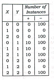 (a) Build a decision tree on the data set. Does the tree capture the ‘+’ and ‘–’ concepts? (b) What are the accuracy, precision, recall and F1-measure of the decision tree? (Note that precision, recall, and F1-measure are defined with respect to the ‘+’ class.)202214m

    Module 3: Classification Algorithms

    Following is a data set that contains two attributes, X and Y, and two class labels, ‘+’ and ‘–’.
    Each attribute can take three different values: 0, 1, or 2.

    The concept for the ‘+’ class is Y = 1
    and the concept for the ‘–’ class is X = 0 ∨ X = 2.

    

    (a)
    Build a decision tree on the data set.
    Does the tree capture the ‘+’ and ‘–’ concepts?

    (b)
    What are the accuracy, precision, recall and F1-measure of the decision tree?
    (Note that precision, recall, and F1-measure are defined with respect to the ‘+’ class.)

    View this question on its own page →

    CopySearch GoogleAsk AI
17. Q6a. Explain the model of over-fitting and under-fitting. Give the example of over-fitting and under-fitting in two-dimensional data.20227m

    Module 1: Introduction

    Explain the model of over-fitting and under-fitting. Give the example of over-fitting and under-fitting in two-dimensional data.

    View this question on its own page →

    CopySearch GoogleAsk AI

    Worked Solution

    Overfitting and Underfitting:

    Overfitting: Model learns training data too well, including noise/outliers; high variance, low bias. Memorization. $Error_{train} \ll Error_{test}$. Example: Degree-10 polynomial fitting 10 points with wiggling curve passing through all points.

    Underfitting: Model too simple to capture underlying pattern; high bias, low variance. $Error_{train} \approx Error_{test}$ but both high. Example: Linear line fitting parabolic data.

    Model complexity view: Train vs Validation error vs capacity (U-shaped test error). Optimal is intermediate capacity (sweet spot) where bias-variance balanced.

    2D Example:

    Data: Parabolic trend $y = x^2 + noise$, points near U-shape.

    • Underfit (linear, degree 1): Straight line cutting through U, misses curvature → large error on both train and test.

      y
      *   *
       \ /     data *
        .      linear ___  (misses curve)
       / \
      *   *
      

    • Good fit (degree 2): Parabola $y= w_0+w_1x+w_2x^2$ captures trend smoothly, generalizes.

    • Overfit (degree 9+): Wiggly curve passing exactly through every noisy point, oscillates wildly between points — zero train error but huge test error.

    Remedies:

    • Underfit: increase complexity, add features, reduce regularization, longer training.
    • Overfit: more data, regularization (L1/L2), pruning, dropout, early stopping, cross-validation, feature selection, reduce degree.

    Visual: Plot $x$ vs $y$, noisy quadratic data; underfit = straight line under, overfit = wiggly interpolating, good = smooth quadratic.

18. Q6b. Explain the bagging and boosting with example.20227m

    Module 3: Classification Algorithms

    Explain the bagging and boosting with example.

    View this question on its own page →

    CopySearch GoogleAsk AI

    Worked Solution

    Bagging and Boosting (Ensemble Methods):

    Both combine weak learners (e.g., decision trees) to strong ensemble but differ in strategy.

    Bagging (Bootstrap Aggregating) — Breiman:

    • Create $M$ bootstrap samples (sample with replacement, size $n$) from training data.
    • Train one base learner on each sample in parallel, e.g., deep trees in Random Forest.
    • Aggregate: Classification majority vote, Regression averaging: $\hat f(x)=\frac1M\sum f_m(x)$
    • Reduces variance, prevents overfitting, robust to noise.
    • Example: Random Forest bagging 100 trees on loan default data, each tree sees 63% unique rows + random feature subset, vote gives stable prediction. Out-of-bag error estimates generalization without CV.

    Boosting (e.g., AdaBoost, Gradient Boosting):

    • Sequential. Train weak learners (stumps) iteratively; each new learner focuses on previously misclassified weighted examples.
    • AdaBoost: Maintain weights $w_i$; initially $1/n$, increase weight for misclassified, decrease for correct. Final prediction weighted vote $F(x)=sign(\sum \alpha_m f_m(x))$ where $\alpha_m=\frac12\ln((1-e_m)/e_m)$.
    • Gradient Boosting: Fits new learner to residual (negative gradient of loss) $r_i = -\partial L(y_i, F_{m-1}(x_i))/\partial F_{m-1}$.
    • Reduces bias (+ variance), converts weak → strong, but prone to overfit if noisy; sequential not easily parallel.

    Comparison:

    	Bagging	Boosting
    Data	Bootstrap subsets	Weighted full data, adaptive
    Training	Parallel, independent	Sequential, dependent
    Reduces	Variance	Bias
    Sensitivity to noise	Robust	Sensitive
    Example learners	Full trees	Shallow stumps

    Example: Bagging on noisy medical data stable; Boosting on same achieves higher accuracy but may overfit unless early stopping/shrinkage.

19. Q7. Discuss the steps in K-means algorithm and evaluate the following table using K-means : 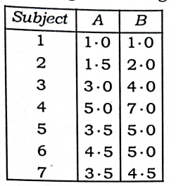202214m

    Module 3: Classification Algorithms

    Discuss the steps in K-means algorithm and evaluate the following table using K-means :

    

    View this question on its own page →

    CopySearch GoogleAsk AI
20. Q8a. What is the difference between K-means and K-medoid algorithm? Explain density-based hierarchical clustering.20227m

    Module 4: Clustering, K-means, K-medoids, Density-based Hierarchical, Spectral .

    What is the difference between K-means and K-medoid algorithm? Explain density-based hierarchical clustering.

    View this question on its own page →

    CopySearch GoogleAsk AI

    Worked Solution

    K-means vs K-medoid:

    Aspect	K-means (Lloyd)	K-medoid (PAM)
    Center	Centroid = mean $\mu_j=\frac1{|C_j|}\sum x$ (not necessarily data point, continuous)	Medoid = actual data point minimizing sum distance to cluster members
    Distance	Euclidean (minimizes SSE)	Any metric (Manhattan, arbitrary dissimilarity)
    Robustness	Sensitive to outliers (mean shifts)	Robust (medoid not affected by extreme outlier)
    Cost function	$J=\sum\sum||x-\mu||^2$	$E=\sum\sum d(x,m_j)$
    Complexity	$O(nkdi)$ fast	$O(k(n-k)^2)$ per iteration (PAM) much slower, $CLARA/CLARANS$ for large data
    When to use	Continuous, spherical clusters, fast	Categorical/mixed, need representatives from dataset, noisy data

    Density-Based Hierarchical Clustering:

    Combines density and hierarchy. Unlike flat K-means, builds tree (dendrogram) where clustering reflects density connectivity at different thresholds.

    • Core idea: Clusters are dense regions separated by sparse regions. Define $\epsilon$-neighborhood and $minPts$. Point types: core (≥$minPts$ in $\epsilon$), border, noise. Hierarchical variant (e.g., HDBSCAN, OPTICS, DENCLUE hierarchical) varies $\epsilon$/density threshold to create hierarchy.

    • OPTICS: Ordering Points To Identify Clustering Structure — computes reachability distance, produces reachability plot, extracts hierarchy without fixing single $\epsilon$.

    • HDBSCAN: Converts DBSCAN to hierarchical, builds minimum spanning tree of mutual reachability, condenses, selects stable clusters via persistence $\lambda=1/distance$.

    • Hierarchical density dendrogram: Bottom leaves = core points merge at lowest density threshold as $\epsilon$ increases.

    Advantages: Finds arbitrary shapes, handles noise, no need to preset $k$, hierarchy reveals clusters at multiple densities.

    Steps generic: Estimate density (kernel), build graph where edges if density > threshold, connected components = clusters, vary threshold → hierarchy, prune unstable branches.

21. Q8b. What is ANN? Explain feed forward and back propagation algorithm with example.20227m

    Module 3: Classification Algorithms

    What is ANN? Explain feed forward and back propagation algorithm with example.

    View this question on its own page →

    CopySearch GoogleAsk AI

    Worked Solution

    Artificial Neural Network (ANN):

    Computational model inspired by biological neurons. Network of interconnected units (neurons) that processes inputs via weighted sums and non-linear activations to learn mappings.

    • Neuron: $net=\sum w_i x_i + b$, $y=f(net)$ where $f$ is activation (sigmoid $1/(1+e^{-net})$, tanh, ReLU $max(0,net)$).
    • Architecture: Input layer → one or more hidden layers → output layer. Fully connected. Depth determines representation power.

    Feedforward Algorithm:
    Information flows forward only, no cycles.

    1. Initialize weights small random.
    2. For each layer $l$: $a^{(l)}=f(W^{(l)}a^{(l-1)}+b^{(l)})$
    3. At output, compute loss $E=\frac12\sum(y-a^{(L)})^2$ or cross-entropy.
    4. Example: 2-input XOR with hidden 2 neurons: $h_1=sigmoid(w_{11}x_1+w_{12}x_2+b_1)$, $output=sigmoid(v_1h_1+v_2h_2+c)$.

    Backpropagation Algorithm:
    Efficient gradient computation via chain rule to train weights.

    1. Forward pass as above, store $net, a$.
    2. Output error $\delta^{(L)}=(y-a^{(L)})f'(net^{(L)})$
    3. Propagate backward: $\delta^{(l)}= (W^{(l+1)T}\delta^{(l+1)})\odot f'(net^{(l)})$
    4. Gradients $\partial E/\partial W^{(l)}=\delta^{(l)}a^{(l-1)T}$
    5. Update $W:=W+\eta\delta a^T$, $b:=b+\eta\delta$ (SGD).
    6. Iterate over epochs until convergence.

    Example with numbers: Single neuron with sigmoid, input 0.5, target 1, $w=0.3$, $net=0.15$, $o=0.537$, $E=0.107$, $\delta=(0.463)*0.248=0.115$, $\Delta w=0.1*0.115*0.5=0.0057$ → weight increases.

    Feedforward computes prediction; backprop assigns blame and updates weights to reduce loss, enabling learning of non-linear boundaries.

22. Budget App•POCKETLY

    Pocketly on Android

    Log daily food, travel, and hostel expenses instantly. Set monthly spending limits and see where your money goes without complex spreadsheets.

    Install Pocketly
23. Q9a. Write short notes on the following: (a) Partial least square20227m

    Module 2: Linear Models and Bayesian Learning

    Write short notes on the following:
    (a) Partial least square

    View this question on its own page →

    CopySearch GoogleAsk AI

    Worked Solution

    (a) Partial Least Squares (PLS):

    PLS is dimensionality reduction + regression method for high-dimensional, multicollinear, $p\gg n$ data (e.g., chemometrics, genomics).

    Goal: Find latent components that maximize covariance between $X$ (predictors) and $Y$ (responses), not just variance of $X$ like PCA.

    Idea: Decompose $X = TP^T + E$, $Y = UQ^T + F$ with $T = XW$, $U = YC$ latent scores, weights $W$ maximize $Cov(T,U) = Corr(T,U) * \sqrt{Var(T)Var(U)}$.

    Algorithm (NIPALS):

    1. Center/scale $X, Y$.
    2. For component $h=1..A$: compute weight $w_h \propto X^T y$ (for univariate $Y$) normalized, $t_h = X w_h$, $p_h = X^T t_h / (t_h^T t_h)$, $q_h = Y^T t_h / (t_h^T t_h)$, deflate $X:= X - t_h p_h^T$, $Y:= Y - t_h q_h^T$.
    3. Regression $Y = T B Q^T$ yields $\hat\beta_{PLS}= W(P^T W)^{-1} B Q^T$.

    Types: PLS1 ($Y$ univariate), PLS2 ($Y$ multivariate), PLS-DA (classification).

    Advantages: Handles multicollinearity, $n<p$, noisy predictors, stable; gives interpretable latent factors (like PCA but supervised).

    Vs PCA/OLS: PCA maximizes $Var(T)$, PLS maximizes $Cov(T,U)$ → better predictive components. OLS fails when $X^T X$ singular; PLS works.

    Choosing components $A$: Cross-validation (Q² metric).

    Example: Predict chemical concentration $Y$ from 1000-wavelength spectra $X$ (highly correlated) with 50 samples → PLS finds 3 latent factors capturing predictive spectra shape.

24. Q9b. Write short notes on the following: (b) Reinforcement learning20227m

    Module 5: Probabilistic & Reinforcement Methods

    Write short notes on the following:
    (b) Reinforcement learning

    View this question on its own page →

    CopySearch GoogleAsk AI

    Worked Solution

    (b) Reinforcement Learning:

    Definition: Paradigm where agent learns optimal policy $\pi^*:S\to A$ by interacting with environment and maximizing cumulative reward, not from labeled examples but from delayed reward signal.

    Components: Agent, Environment, State $s$, Action $a$, Reward $r$, Policy $\pi$, Value $V^\pi, Q^\pi$, Model $p(s'|s,a)$, discount $\gamma$.

    Types:

    • Model-free: No explicit model; directly learn $V/Q/\pi$. Value-based (Q-learning $Q(s,a)\leftarrow Q+\alpha[r+\gamma\max Q(s',a')-Q]$), Policy-based (REINFORCE $
      abla J=E[
      abla\log\pi(a|s) Q]$), Actor-Critic.
    • Model-based: Learn/know $p(s'|s,a)$, plan via DP (Value Iteration, MCTS in AlphaGo).
    • On-policy (SARSA) learns about $\pi$ being followed; off-policy (Q-learning) learns about optimal $\pi$ from any behavior.

    Exploration-Exploitation: $\epsilon$-greedy, UCB, Thompson, entropy regularization.

    Algorithms: Q-learning, SARSA, DQN (deep $Q$ with replay + target network), Policy Gradient, PPO, A3C.

    Challenges: Credit assignment (delayed reward), exploration, instability, sample inefficiency.

    Applications: Game playing (AlphaGo, Atari DQN), robotics control, autonomous driving, recommender systems (long-term engagement), finance trading.

    Example: Grid maze: states = cells, actions = up/down/left/right, reward +10 goal, -1 wall, agent via Q-learning propagates values back from goal to learn shortest path.

    Differences vs supervised: No correct output provided, only reward; sequential, action affects next state (non-i.i.d).

    Rewards shape behavior; reward engineering crucial.