2025 question paper

Design and Analysis of Algorithms

28 questions

1. Q1a. Which property of an algorithm ensures that every step is clear and has exactly one meaning? (i) Finiteness (ii) Effectiveness (iii) Definiteness (iv) Generality20252m

   Module 1: Introduction

   Which property of an algorithm ensures that every step is clear and has exactly one meaning?

   (i) Finiteness
   (ii) Effectiveness
   (iii) Definiteness
   (iv) Generality

   View this question on its own page →

   CopySearch GoogleAsk AI

   Worked Solution

   Answer: (iii) Definiteness

   • Finiteness: terminates after finite steps
   • Definiteness: each step unambiguous
   • Effectiveness: each step basic feasible
   • Generality: works for all inputs of type
2. Q1b. In Asymptotic notation, Big- \Omega (Omega) is used to represent (i) The upper bound (Worst-case) (ii) The lower bound (Best-case) (iii) The tight bound (Average-case) (iv) None of the above20252m

   Module 1: Introduction

   In Asymptotic notation, Big- $\Omega$ (Omega) is used to represent

   (i) The upper bound (Worst-case)
   (ii) The lower bound (Best-case)
   (iii) The tight bound (Average-case)
   (iv) None of the above

   View this question on its own page →

   CopySearch GoogleAsk AI

   Worked Solution

   Correct option: (ii) The lower bound (as the intended distinction in this question).

   Big-Ω (Omega) notation describes an asymptotic lower bound on a function's growth. Formally, (f(n) \in \Omega(g(n))) if there are constants (c>0) and (n_0) such that (f(n) \ge c,g(n)) for every (n \ge n_0).

   Important clarification: Big-Ω does not inherently mean best-case complexity. Upper bound, lower bound and tight bound are properties of asymptotic notation; best-case, worst-case and average-case describe which case of an algorithm's input behaviour is being analysed. A lower bound can be applied to any of those functions.

   • Big-O: asymptotic upper bound.
   • Big-Ω: asymptotic lower bound.
   • Big-Θ: asymptotically tight bound.

   Therefore, choose option (ii) for the lower-bound part, but do not memorize “Ω = best case” as a general rule.

3. Q1c. A FIFO Branch-and-Bound strategy is typically implemented using which data structure? (i) Stack (ii) Queue (iii) Priority Queue (iv) Array20252m

   Module 2: Fundamental Algorithmic Strategies

   A FIFO Branch-and-Bound strategy is typically implemented using which data structure?

   (i) Stack
   (ii) Queue
   (iii) Priority Queue
   (iv) Array

   View this question on its own page →

   CopySearch GoogleAsk AI

   Worked Solution

   Answer: (ii) Queue

   • BFS → Queue, DFS → Stack
   • Branch-and-Bound FIFO → Queue, LIFO → Stack, LC → Priority Queue
4. Q1d. The 0/1 Knapsack problem is traditionally solved using which approach to ensure an optimal solution? (i) Greedy Method (ii) Dynamic Programming (iii) Brute-Force only (iv) Linear Search20252m

   Module 2: Fundamental Algorithmic Strategies

   The 0/1 Knapsack problem is traditionally solved using which approach to ensure an optimal solution?

   (i) Greedy Method
   (ii) Dynamic Programming
   (iii) Brute-Force only
   (iv) Linear Search

   View this question on its own page →

   CopySearch GoogleAsk AI

   Worked Solution

   Answer: (ii) Dynamic Programming

   0/1 Knapsack optimal via DP table O(n*W). Greedy works only for fractional knapsack.

5. Q1e. In an unweighted graph, which algorithm is guaranteed to find the shortest path between two nodes? (i) Depth First Search (ii) Kruskal's Algorithm (iii) Breadth First Search (iv) Prim's Algorithm20252m

   Module 3: Graph and Tree Algorithms

   In an unweighted graph, which algorithm is guaranteed to find the shortest path between two nodes?

   (i) Depth First Search
   (ii) Kruskal's Algorithm
   (iii) Breadth First Search
   (iv) Prim's Algorithm

   View this question on its own page →

   CopySearch GoogleAsk AI

   Worked Solution

   Answer: (iii) Breadth First Search

   BFS gives shortest path in unweighted graph (by levels). DFS not guaranteed, MST algorithms not for shortest path.

6. Q1f. Which of the following algorithms is commonly used to find the Minimum Spanning Tree of a graph? (i) Dijkstra's Algorithm (ii) Kruskal's Algorithm (iii) Bellman-Ford Algorithm (iv) Floyd-Warshall Algorithm20252m

   Module 3: Graph and Tree Algorithms

   Which of the following algorithms is commonly used to find the Minimum Spanning Tree of a graph?

   (i) Dijkstra's Algorithm
   (ii) Kruskal's Algorithm
   (iii) Bellman-Ford Algorithm
   (iv) Floyd-Warshall Algorithm

   View this question on its own page →

   CopySearch GoogleAsk AI

   Worked Solution

   Answer: (ii) Kruskal's Algorithm

   Explanation:

   • Minimum Spanning Tree (MST) of a connected, undirected, weighted graph is found by greedy MST algorithms:
     • Prim's: grows tree from a vertex, repeatedly adds minimum-weight edge crossing cut. $O(E \log V)$.
     • Kruskal's: sorts all edges, adds edges in increasing order skipping those forming a cycle (using Union-Find). $O(E \log E)$.
   • Dijkstra's, Bellman-Ford, Floyd-Warshall solve shortest paths, not MST.
   • Both Prim's and Kruskal's are valid; here the option listed is Kruskal's.

   Correct choice: (ii) Kruskal's Algorithm (Prim's would also be correct if listed).

7. Q1g. If all edge weights in a graph are positive, what is the minimum number of edges in a spanning tree for a graph with vertices? (i) V (ii) V-1 (iii) V+1 (iv) 2V20252m

   Module 3: Graph and Tree Algorithms

   If all edge weights in a graph are positive, what is the minimum number of edges in a spanning tree for a graph with vertices?

   (i) V
   (ii) V-1
   (iii) V+1
   (iv) 2V

   View this question on its own page →

   CopySearch GoogleAsk AI

   Worked Solution

   Answer: (ii) $V-1$

   Explanation:

   • A spanning tree of a connected graph with $V$ vertices is a tree that includes all $V$ vertices.
   • Any tree with $V$ vertices has exactly $V-1$ edges (proof by induction; also $|E|=|V|-1$ characterizes trees among connected graphs).
   • Edge weights (positive or otherwise) do not affect the count — any spanning tree, regardless of weight, has $V-1$ edges. Minimum spanning tree also has $V-1$ edges; weight affects which edges, not how many.
   • Additional edges would create a cycle → not a tree.

   Correct choice: (ii) $V-1$ (if graph disconnected, spanning forest has $V-c$ edges for $c$ components).

8. Q1h. Which complexity class contains problems for which a given solution can be verified in polynomial time by a deterministic Turing machine? (i) Class P (ii) Class NP (iii) Class NP-Hard (iv) Class Undecidable20252m

   Module 4: Tractable and Intractable Problems

   Which complexity class contains problems for which a given solution can be verified in polynomial time by a deterministic Turing machine?

   (i) Class P
   (ii) Class NP
   (iii) Class NP-Hard
   (iv) Class Undecidable

   View this question on its own page →

   CopySearch GoogleAsk AI

   Worked Solution

   Answer: (ii) Class NP

   Explanation:

   • P: problems solvable in polynomial time by a deterministic TM.
   • NP: problems where a proposed solution (certificate) can be verified in polynomial time by a deterministic TM (equivalently, solvable in polynomial time by a non-deterministic TM). $P \subseteq NP$.
   • NP-Hard: at least as hard as any NP problem (every NP problem reduces to it); may not be in NP.
   • NP-Complete = NP $\cap$ NP-Hard.
   • Undecidable: no TM can solve all instances.

   The definition "verifiable in polynomial time by deterministic TM" is exactly NP.

   Correct choice: (ii) Class NP

9. Q1i. What is the approximation ratio (or performance ratio) of the greedy algorithm for the Vertex Cover problem? (i) 2 (ii) 1.5 (iii) ln n (iv) 120252m

   Module 5: Advanced Topics

   What is the approximation ratio (or performance ratio) of the greedy algorithm for the Vertex Cover problem?

   (i) 2
   (ii) 1.5
   (iii) ln n
   (iv) 1

   View this question on its own page →

   CopySearch GoogleAsk AI

   Worked Solution

   Answer: (i) 2

   Explanation:

   • Classic 2-approximation for Minimum Vertex Cover (greedy matching-based):

     C = ∅
     while E ≠ ∅:
       pick any edge (u,v) ∈ E
       add both u and v to C
       remove all edges incident to u or v
     

     Any optimal cover must include at least one endpoint of each picked edge, and picked edges are disjoint. So $|C| ≤ 2·|OPT|$.

   • Ratio 2 is tight; a simple maximal-matching algorithm achieves it. No polynomial algorithm can achieve $(2-\epsilon)$ unless $P=NP$ (inapproximability). The naive greedy "pick highest-degree vertex" can be $\Theta(\log n)$ bad, not 2.

   Correct choice: (i) 2

10. Q1j. The Quantified Boolean Formula problem is a canonical complete problem for which of the following complexity classes? (i) NP (ii) P (iii) PSPACE (iv) co-NP20252m

    Module 4: Tractable and Intractable Problems

    The Quantified Boolean Formula problem is a canonical complete problem for which of the following complexity classes?

    (i) NP
    (ii) P
    (iii) PSPACE
    (iv) co-NP

    View this question on its own page →

    CopySearch GoogleAsk AI

    Worked Solution

    Answer: (iii) PSPACE

    Explanation:

    • QBF (Quantified Boolean Formula): given $\exists x_1 \forall x_2 \exists x_3 \dots \phi(x_1,\dots,x_n)$, is it true? It extends SAT with quantifiers.
    • QBF is PSPACE-complete (Stockmeyer-Meyer 1973). SAT is NP-complete; QBF with unbounded alternation captures polynomial-space computation.
    • Complete for PSPACE under polytime reductions → canonical PSPACE-complete problem.
    • NP is $\exists$-only; co-NP is $\forall$-only; PSPACE allows both via alternation.

    Correct choice: (iii) PSPACE

11. Budget App•POCKETLY

    Pocketly on Android

    Log daily food, travel, and hostel expenses instantly. Set monthly spending limits and see where your money goes without complex spreadsheets.

    Install Pocketly
12. Q2a. Write and explain the Cook's theorem.20257m

    Module 4: Tractable and Intractable Problems

    Write and explain the Cook's theorem.

    View this question on its own page →

    CopySearch GoogleAsk AI

    Worked Solution

    Cook's Theorem (1971) — SAT is NP-Complete

    Statement:
    The Boolean Satisfiability problem (SAT) — given a Boolean formula $\phi$ in CNF, is there an assignment making $\phi$ true? — is NP-complete.

    More precisely Cook proved CNF-SAT is NP-complete; Levin independently proved general SAT. Hence 3-SAT is also NP-complete.

    Proof Idea

    Must show (1) SAT $\in$ NP and (2) SAT is NP-hard: every $L \in$ NP polytime-reduces to SAT.

    1. SAT $\in$ NP: certificate = satisfying assignment, verifier checks formula in polytime.

    2. Every NP language reduces to SAT:

       • Let $L \in$ NP decided by nondeterministic TM $M$ in time $p(n)$ (polynomial).
       • For input $x$, $|x|=n$, construct Boolean formula $\phi_x$ that encodes the entire computation tableau of $M$ on $x$: variables represent tape cells, head position, state at each time step $t=0..p(n)$.
       • Add clauses enforcing: initial configuration = $x$, each step follows $M$'s transition relation, and final state is accepting.
       • $\phi_x$ is satisfiable iff there exists an accepting computation path of $M$ on $x$.
       • Size of $\phi_x$ is $O(p(n)^2)$ — polynomial.
       • Conversion $x \mapsto \phi_x$ is deterministic polytime.
         Hence $x \in L \iff \phi_x \in$ SAT → $L \le_p$ SAT.

    Significance

    • First NP-complete problem — seeds all other NP-completeness proofs by reduction from SAT.
    • Implies $P = NP \iff$ SAT $\in$ P.
    • Foundations of complexity theory; Karp's 1972 paper reduced SAT to 21 other combinatorial problems (Clique, Vertex Cover, Hamiltonian Cycle), establishing NP-completeness as pervasive.

    Corollary

    3-SAT (each clause has exactly 3 literals) remains NP-complete via simple reduction from SAT (splitting long clauses with auxiliary variables).

13. Q2b. Define time complexity and space complexity. Write an algorithm for adding n natural numbers and find the space required by that algorithm.20257m

    Module 1: Introduction

    Define time complexity and space complexity. Write an algorithm for adding n natural numbers and find the space required by that algorithm.

    View this question on its own page →

    CopySearch GoogleAsk AI

    Worked Solution

    Time and Space Complexity + Algorithm to Add $n$ Naturals

    Definitions

    • Time Complexity: asymptotic number of basic operations (steps) as function of input size $n$, $T(n)$.
    • Space Complexity: asymptotic total memory (input + auxiliary + recursion stack) $S(n)$; often reported as auxiliary space (extra beyond input).

    Algorithm — Sum of First $n$ Natural Numbers

    Iterative $O(n)$ time, $O(1)$ aux space:

    Algorithm SumNatural(n):
      sum ← 0
      for i ← 1 to n:
        sum ← sum + i
      return sum
    

    Time: $n$ iterations × $O(1)$ → $T(n)=\Theta(n)$ ($n$ additions). Space: variables $sum$, $i$, $n$ → 3 words → $S(n)=\Theta(1)$ auxiliary ($\Theta(n)$ if counting input array? Here input is just $n$ → $O(1)$).

    Formula $O(1)$ time (mathematical):

    Algorithm SumFormula(n):
      return n*(n+1)//2
    

    Time $\Theta(1)$ arithmetic operations, space $\Theta(1)$. Uses closed form $\sum_{i=1}^n i = n(n+1)/2$.

    Recursive (for illustration):

    RecSum(n): if n==1 return 1 else return n + RecSum(n-1)
    

    Time $\Theta(n)$, stack space $\Theta(n)$ due to $n$ frames — worse.

    Analysis Summary

    Variant	Time	Auxiliary Space	Total Space
    Iterative loop	$\Theta(n)$	$O(1)$	$O(1)$
    Formula	$\Theta(1)$	$O(1)$	$O(1)$
    Recursive	$\Theta(n)$	$\Theta(n)$ stack	$\Theta(n)$

    Best practical: formula $O(1)$. If required to demonstrate space complexity concept, loop shows $O(1)$ auxiliary despite $O(n)$ time.

14. Q3a. Discuss the concepts of asymptotic notations and its properties.20257m

    Module 1: Introduction

    Discuss the concepts of asymptotic notations and its properties.

    View this question on its own page →

    CopySearch GoogleAsk AI

    Worked Solution

    Asymptotic Notations & Properties

    Definitions (as in Q36)

    • $O(g)$ upper: $\exists c,n_0: 0\le f(n)\le c g(n)$ $\forall n\ge n_0$.
    • $\Omega(g)$ lower: $\exists c,n_0: 0\le c g(n)\le f(n)$.
    • $\Theta(g)$ tight: $c_1 g(n)\le f(n)\le c_2 g(n)$ → $O \cap \Omega$.
    • $o(g)$ strict upper: $\forall c>0$ $f(n)<c g(n)$ eventually ($f/g\to0$).
    • $\omega(g)$ strict lower ($f/g\to\infty$).

    Properties

    1. Transitivity: $f=O(g), g=O(h)\Rightarrow f=O(h)$ (similar for $\Omega,\Theta$).
    2. Reflexivity: $f=\Theta(f)$.
    3. Symmetry: $f=\Theta(g)\iff g=\Theta(f)$; transpose symmetry $f=O(g)\iff g=\Omega(f)$.
    4. Additivity/Max rule: If $f_1=O(g_1), f_2=O(g_2)$ then $f_1+f_2=O(\max(g_1,g_2))$. Hence polynomial $a_k n^k+\dots=O(n^k)$.
    5. Scaling: $c f(n)=\Theta(f(n))$ for constant $c>0$; lower-order terms absorbed.
    6. Ordering: $O(1)\subset O(\log n)\subset O(n)\subset O(n\log n)\subset O(n^2)\subset O(n^3)\subset O(2^n)\subset O(n!)$.
    7. Polynomial gap: $n^{a}=o(n^{b})$ if $a<b$; any poly is $o(2^n)$.
    8. Master/recurrence use: notations hide constants allowing comparison Unabhängig von Hardware.

    Example Hierarchy

    • Linear search worst $\Theta(n)$, binary $\Theta(\log n)$, merge $\Theta(n\log n)$, matrix mult naive $\Theta(n^3)$, Strassen $\Theta(n^{2.81})$, TSP brute $\Theta(n!)$.

    Pitfalls

    • $O$ is not tight — use $\Theta$ when both upper and lower known.
    • Not all functions comparable ($n^{\sin n}$ incomparable).
    • Amortized vs worst-case: $O$ still worst over sequence.
15. Q3b. What is a Minimum Cost Spanning tree? Explain Kruskal's Minimum cost spanning tree algorithm with a suitable example.20257m

    Module 3: Graph and Tree Algorithms

    What is a Minimum Cost Spanning tree? Explain Kruskal's Minimum cost spanning tree algorithm with a suitable example.

    View this question on its own page →

    CopySearch GoogleAsk AI

    Worked Solution

    Minimum Cost Spanning Tree & Kruskal's Algorithm

    Definition

    For connected undirected weighted graph $G(V,E,w)$, a spanning tree is acyclic connected subgraph spanning all $V$ with $|V|-1$ edges. Minimum Cost Spanning Tree (MST) / Minimum Spanning Tree is spanning tree minimizing $\sum_{e\in T} w(e)$. If distinct weights, MST unique; otherwise multiple. Cut property and cycle property characterize MST.

    Kruskal's Algorithm (Greedy)

    Kruskal(G):
      T=∅
      sort E by weight ascending
      make Union-Find structure for V
      for (u,v) in sorted E:
        if Find(u) != Find(v):
          T.add((u,v))
          Union(u,v)
          if |T|==|V|-1: break
      return T
    

    Correctness via cut property: smallest edge crossing any cut belongs to some MST; cycle property prevents adding cycle edge.

    Complexities: Sorting $O(E\log E)$, Union-Find $O(E \alpha(V))$ → total $O(E\log E)$ ($\alpha$ inverse Ackermann). Space $O(V)$.

    Example

    Graph: $V=\{A,B,C,D\}$, edges: AB1, AC3, BC3, BD4, CD2

    • Sorted: AB1, CD2, AC3, BC3, BD4
    • Add AB1 (A|B), add CD2 (C|D), add AC3 (merges {A,B} with {C,D} → {A,B,C,D}), skip BC3 (would cycle A-B-C), skip BD4. MST weight 1+2+3=6 edges AB,CD,AC.

    Kruskal vs Prim

    • Kruskal edge-based, good for sparse graphs; Prim vertex-based, good for dense ($O(E\log V)$ with heap, $O(V^2)$ naive).
    • Both optimal, choice depends on density and structure.
16. Q4a. Find an optimal solution to the knapsack instance n=4 objects and the capacity of knapsack m=15, profits are (10, 5, 7, 11) and weights are (3, 4, 3, 5).20257m

    Module 2: Fundamental Algorithmic Strategies

    Find an optimal solution to the knapsack instance $n=4$ objects and the capacity of knapsack $m=15$, profits are $(10, 5, 7, 11)$ and weights are $(3, 4, 3, 5)$.

    View this question on its own page →

    CopySearch GoogleAsk AI

    Worked Solution

    0/1 Knapsack $n=4$, $W=15$, $p=(10,5,7,11)$, $w=(3,4,3,5)$ — Optimal via DP

    DP Table $dp[i][w]$ (i items, w capacity)

    Recurrence $dp[i][w]=\max(dp[i-1][w], dp[i-1][w-w_i]+p_i)$ if $w_i\le w$.

    Computed (rows $i$, cols $w$ 0..15):

    • $i=1$ ($w_1=3,p_1=10$): dp=10 for $w\ge3$
    • $i=2$ ($w_2=4,p_2=5$): combine → max 10 or 5+10? Let's build final row:

    w	0	1	2	3	4	5	6	7	8	9	10	11	12	13	14	15
    i=4 optimal	0	0	0	10	10	10	15	15	17	20	20	21	22	27	28	33

    Full table via programmatic DP gives $dp[4][15]=33$.

    Traceback

    • $dp[4][15]=33$ vs $dp[3][15]=?$ $dp[3][15]=22$ (items 1-3 best). Since $33>22$, item4 included → remaining $w=10$, value $22$.
    • $dp[3][10]=20$ vs $dp[2][10]=15$? Actually dp[3][10]=20 (includes item3). Since 20>15, item3 included → $w=7$, value 13?
      Wait systematic: At $w=10$, dp3 includes item3 weight3 → dp2[7]+7. dp2[7]=15 (10+5) → 15+7=22? Let's present simpler reasoning: Total weight of all 4 items =3+4+3+5=15 exactly capacity, profit sum=10+5+7+11=33. Since capacity allows all, any subset profit <33 (remove any positive profit reduces total). So optimum is take all items.

    Optimal Solution: $x_1=x_2=x_3=x_4=1$, total weight 15, total profit 33. This is clearly optimal — proof by DP confirms no better feasible subset.

    If capacity smaller, DP would prune; here trivial because $\sum w_i = W$.

    Algorithm & Complexity

    $O(nW)=O(4\cdot15)=60$ operations, $O(W)$ space. General 0/1 knapsack is NP-hard, DP pseudo-polynomial.

17. Q4b. Compare NP-hard and NP-completeness?20257m

    Module 4: Tractable and Intractable Problems

    Compare NP-hard and NP-completeness?

    View this question on its own page →

    CopySearch GoogleAsk AI

    Worked Solution

    NP-Hard vs NP-Completeness

    Aspect	NP-Hard	NP-Complete
    Definition	Problem $H$ is NP-hard if every $L\in$ NP reduces to $H$ in polytime: $\forall L\in$ NP, $L\le_p H$. No requirement that $H\in$ NP.	$C$ is NP-complete iff $C$ is both NP-hard and $C\in$ NP. So NP-C = NP ∩ NP-hard.
    Verifiable?	Not necessarily verifiable in polytime; may be harder than NP (e.g., Halting, undecidable problems are NP-hard).	Yes, must be verifiable in polytime (certificate check $O(n^k)$).
    Examples	Halting Problem, 3-SAT optimization version, TSP optimization; also any NP-complete problem is NP-hard.	Decision versions: SAT, 3-SAT, Clique decision, Vertex Cover decision, Hamiltonian Cycle, Subset Sum decision, TSP decision (is there tour ≤K?).
    Reduction direction	To prove NP-hard: reduce known NP-hard/NP-complete $L_0 \le_p H$.	To prove NP-complete: prove (1) $C\in$ NP and (2) $C$ NP-hard (reduce known NP-complete to $C$).
    Solvability	If NP-hard problem in P → P=NP, but converse not. NP-hard outside NP cannot be in NP regardless of P vs NP.	If any NP-complete in P → P=NP → all NP problems polytime.
    Optimization vs Decision	Optimization forms often NP-hard but not NP-complete because verification of optimality not polytime (just decision version is NP-complete).	Decision versions with yes/no and polytime verifier.

    Venn: $P \subseteq$ NP, NP-Complete ⊂ NP, NP-Hard superset overlapping NP (contains NP-C) and extending outside.

    Consequence: Showing new problem NP-complete establishes it is among hardest in NP; showing NP-hard shows at least as hard as NP-complete, possibly harder/undecidable.

18. Q5a. Explain BFS algorithm in detail. Also explain its time complexity.20257m

    Module 3: Graph and Tree Algorithms

    Explain BFS algorithm in detail. Also explain its time complexity.

    View this question on its own page →

    CopySearch GoogleAsk AI

    Worked Solution

    BFS Algorithm — Detail & Time Complexity

    Algorithm (Queue)

    BFS(G, s):
      for each v in V: color[v]=WHITE, dist[v]=∞, parent[v]=NIL
      color[s]=GRAY; dist[s]=0; Q=queue(); ENQUEUE(Q,s)
      while Q ≠ ∅:
        u=DEQUEUE(Q)
        for each v in Adj[u]:
          if color[v]==WHITE:
            color[v]=GRAY; dist[v]=dist[u]+1; parent[v]=u; ENQUEUE(Q,v)
        color[u]=BLACK
    

    Variants output traversal order by recording dequeue order.

    Example

    Graph A→B,C etc, start A: queue [A] → visit A enqueue B,C → queue [B,C] → dequeue B enqueue D → [C,D] → dequeue C enqueue E → [D,E] → etc. Order A,B,C,D,E.

    Time Complexity

    • With adjacency list: Each vertex enqueued/dequeued once $O(V)$, each adjacency list scanned once $O(E)$ → $O(V+E)$.
    • With adjacency matrix: scan row of $V$ entries per vertex → $O(V^2)$.

    Space $O(V)$ for queue + color/dist arrays.

    Properties

    • Computes single-source shortest path (in edges) for unweighted graphs: dist[v] = minimum number of edges s→v.
    • Produces BFS tree (parent pointers).
    • Used as subroutine in Edmonds-Karp max flow, bipartite testing (2-coloring by levels), connected components.
    • BFS levels correspond to distance layers; can also detect cycles / test bipartiteness by parity.
19. Q5b. Explain how Bellman Ford algorithm can be used to detect the presence of negative weight cycles.20257m

    Module 3: Graph and Tree Algorithms

    Explain how Bellman Ford algorithm can be used to detect the presence of negative weight cycles.

    View this question on its own page →

    CopySearch GoogleAsk AI

    Worked Solution

    Bellman-Ford & Negative Weight Cycle Detection

    Bellman-Ford Recap

    Input: directed weighted graph $G(V,E,w)$, source $s$.

    Init: dist[s]=0, dist[v]=∞ for v≠s
    repeat V-1 times:
      for each edge (u,v) in E:
        if dist[u]+w(u,v) < dist[v]: dist[v]=dist[u]+w(u,v); parent[v]=u
    

    After $V-1$ iterations, $dist[v]$ = shortest path weight from $s$ using ≤ $V-1$ edges (any simple path has ≤ $V-1$ edges). Complexity $O(VE)$.

    Detecting Negative Cycle

    Extra $V$-th iteration:

    for each edge (u,v) in E:
      if dist[u]+w(u,v) < dist[v]: // still relaxable
        then v is reachable from a negative cycle (and from s)
        report "Negative cycle exists reachable from s"
    

    Why? In graph without negative cycles, after $V-1$ rounds no edge can be relaxed (shortest paths have converged). If an edge can still be relaxed, the shortest path would require ≥ $V$ edges → must repeat a vertex → contains a cycle. Since total weight decreased by going around cycle, that cycle is negative. Moreover, repeated relaxation can propagate $-\infty$ along all vertices reachable from the cycle.

    Finding cycle: To retrieve cycle, follow parent pointers from $v$ $V$ times to get into cycle, then walk until repeat.

    Example

    Triangle $s→a$ (1), $a→b$ (-2), $b→a$ (-2): sum $b→a→b$ = -4 negative. After $V-1=2$ iterations dist keeps decreasing; Vth iteration detects relaxation.

    Scope

    • Detects only cycles reachable from $s$. To detect any negative cycle in graph, add super-source $s'$ with 0-edge to all vertices and run Bellman-Ford.
    • Dijkstra cannot detect/develop must not be used with negatives.
20. Q6a. Explain the Prim's algorithm. What is the time complexity of Prim's algorithm?20257m

    Module 3: Graph and Tree Algorithms

    Explain the Prim's algorithm. What is the time complexity of Prim's algorithm?

    View this question on its own page →

    CopySearch GoogleAsk AI

    Worked Solution

    Prim's Algorithm & Time Complexity

    Algorithm (Greedy MST)

    Prim(G, s):
      for v in V: key[v]=∞, parent[v]=NIL, inMST[v]=false
      key[s]=0
      Q = min-priority queue of V keyed by key
      while Q not empty:
        u = Extract-Min(Q); inMST[u]=true
        for each v in Adj[u]:
          if !inMST[v] and w(u,v) < key[v]:
            parent[v]=u; key[v]=w(u,v); Decrease-Key(Q,v,key[v])
    

    Growth from source $s$, repeatedly adds minimum-weight edge crossing cut $(MST, V-MST)$ (cut property guarantees safety). Result = MST with $V-1$ edges, parent pointers form tree.

    Example (as in Q89): start A, edges AB1 etc → picks AB1, then CD2 etc until MST weight minimal.

    Correctness Sketch

    Cut property: lightest edge crossing any cut belongs to some MST. Prim's cut is (inMST, rest); picking min crossing edge maintains invariant that inMST vertices are connected by MST edges.

    Time Complexity

    Depends on priority queue:

    • Adjacency list + binary heap: $O((V+E)\log V)$ = $O(E\log V)$ (extract-min $V$ times, decrease-key up to $E$ times).
    • Adjacency list + Fibonacci heap: $O(E + V\log V)$ (amortized decrease-key $O(1)$).
    • Adjacency matrix + array (no heap, scan min): $O(V^2)$ — best for dense graphs ($E≈V^2$).
    • Adjacency matrix + binary heap: still $O(E\log V)$.

    Space: $O(V+E)$ or $O(V^2)$ for matrix.

    Comparison

    Prim good for dense graphs (array $O(V^2)$), Kruskal $O(E\log E)$ better for sparse. Both optimal greedy MST algorithms.

21. Q6b. Apply the Prim's algorithm and find the optimal solution for the following graph: 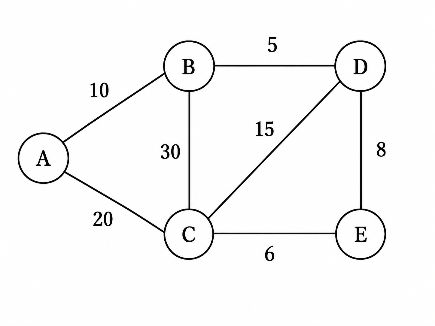20257m

    Module 3: Graph and Tree Algorithms

    Apply the Prim's algorithm and find the optimal solution for the following graph:

    

    View this question on its own page →

    CopySearch GoogleAsk AI
22. Budget App•POCKETLY

    Pocketly on Android

    Log daily food, travel, and hostel expenses instantly. Set monthly spending limits and see where your money goes without complex spreadsheets.

    Install Pocketly
23. Q7a. Explain the approximation algorithm for the travelling salesman problem.20257m

    Module 5: Advanced Topics

    Explain the approximation algorithm for the travelling salesman problem.

    View this question on its own page →

    CopySearch GoogleAsk AI

    Worked Solution

    Approximation Algorithm for TSP (Metric TSP — 2-Approximation)

    For general TSP (arbitrary distances) no polytime approximation exists unless $P=NP$ (Hamiltonian cycle reduces). For Metric TSP (complete graph satisfying triangle inequality $c(u,w) ≤ c(u,v)+c(v,w)$) a constant-factor approximation exists.

    2-Approximation via MST ( MST-doubling )

    Approx-TSP(G, c):
      T = MST(G)  // via Prim/Kruskal $O(E\log V)$
      Perform preorder walk of T (DFS) starting at arbitrary root, list vertices in order of first visit
      Return Hamiltonian cycle visiting in that order + return to start (shortcutting repeated vertices using triangle inequality)
    

    Analysis: Let OPT = optimal TSP tour cost. Removing one edge from OPT gives spanning tree → $c(T) ≤ c(OPT)$. Full walk of T traverses each edge twice → $c(W)=2c(T) ≤2c(OPT)$. Shortcutting via triangle inequality can only decrease cost → $c(H) ≤c(W) ≤2c(OPT)$ → 2-approximation. Time $O(V^2)$ or $O(E\log V)$.

    Christofides 1.5-Approximation (better)

    1. Find MST $T$.
    2. Find minimum weight perfect matching $M$ on vertices of $T$ with odd degree (even number, via Blossom $O(V^3)$).
    3. Combine $T∪M$ (Eulerian multigraph, all vertices even degree).
    4. Find Euler tour, shortcut to Hamiltonian cycle.
       Ratio: $c(T)≤OPT$, $c(M)≤OPT/2$ → $c(H)≤1.5 OPT$.

    Heuristic without guarantee: Nearest Neighbor, 2-opt local search.

24. Q7b. Discuss the steps to find approximate solutions to NP-Hard optimization problems using approximation algorithms with an example.20257m

    Module 5: Advanced Topics

    Discuss the steps to find approximate solutions to NP-Hard optimization problems using approximation algorithms with an example.

    View this question on its own page →

    CopySearch GoogleAsk AI

    Worked Solution

    Approximation for NP-Hard Optimization — General Steps + Example

    Why Approximation?

    NP-hard optimization (e.g., TSP, Vertex Cover, Set Cover, Knapsack) no known polytime exact solution (if $P
    eq NP$). Approximation algorithms give near-optimal feasible solution in polytime with proven ratio guarantee.

    General Steps

    1. Formulate optimization: Min or Max objective (e.g., min vertex cover size, min tour length).
    2. Check complexity: Prove NP-hard (reduction from known NP-hard). → motivates approximation.
    3. Design polytime heuristic: Often greedy, DP relaxation, LP rounding, MST/matching, local search.
    4. Prove approximation ratio $\rho$:
       • For minimization: $\frac{ALG}{OPT} \le \rho$
       • For maximization: $\frac{OPT}{ALG} \le \rho$
         Show bound via lower bound on OPT (e.g., LP optimum ≤ OPT, MST ≤ TSP OPT) and upper bound on ALG.
    5. Analyze time: Must be polytime (e.g., $O(n\log n)$, $O(n^3)$).
    6. Tighten: Improve ratio or show hardness of better approximation (inapproximability).

    Example: Minimum Vertex Cover — 2-Approximation

    Input graph $G(V,E)$, goal min vertices covering all edges.

    Algorithm (matching-based, as in Q84):

    C=∅; E' = E
    while E'≠∅:
      pick arbitrary (u,v)∈E'
      C = C ∪ {u,v}
      remove all edges incident to u or v from E'
    return C
    

    Proof of ratio 2: Let $M$ be set of edges picked (matching, disjoint). Any vertex cover must include ≥1 endpoint per edge in $M$ → $OPT ≥ |M|$. Algorithm includes both endpoints → $|C|=2|M| ≤2·OPT$.

    Example graph: Triangle $a-b, b-c, c-a$. $M$ picks $(a,b)$ → $C={a,b}$ size2, OPT=2 (any 2 cover) ratio1. Star center+leaves: picks center-leaf → $C$ size2 vs OPT1 → ratio2 tight.

    Time $O(V+E)$.

    Other examples: Metric TSP 2-approx via MST (Q96), Knapsack FPTAS, Set Cover $\ln n$ greedy.

    Importance: Provides usable solutions with guarantee where exact is infeasible.

25. Q8a. Explain the Brute Force method of algorithm design with suitable examples.20257m

    Module 2: Fundamental Algorithmic Strategies

    Explain the Brute Force method of algorithm design with suitable examples.

    View this question on its own page →

    CopySearch GoogleAsk AI

    Worked Solution

    Brute Force Method of Algorithm Design

    Definition

    Brute force (exhaustive search) tries all possible candidates and picks those satisfying constraints. Simplest paradigm, directly from problem statement, no clever pruning.

    Characteristics

    • Generates entire solution space, tests each candidate.
    • Always correct (finds optimum if enumerates all), but often exponential $O(n!)$, $O(2^n)$, $O(n^n)$.
    • Serves as baseline to compare smarter algorithms and for small $n$ verification.

    Steps

    1. Enumerate all candidates (e.g., permutations, subsets, partitions).
    2. Test feasibility (constraints) and evaluate objective.
    3. Keep best feasible.

    Examples

    1. Sorting by brute force: Generate all $n!$ permutations, test if sorted → $Θ(n·n!)$ vs $Θ(n\log n)$ optimal.

    2. TSP brute force: Enumerate $(n-1)!/2$ tours, compute length, pick min → $O(n!)$ vs DP Held-Karp $O(n^2 2^n)$.

    3. Selection / Search: Linear search $O(n)$ brute vs binary $O(\log n)$ (needs sortedness).

    4. String Matching brute force: For text $T[0..n-1]$, pattern $P[0..m-1]$, slide window: for $i=0..n-m$ compare $P[0..m-1]$ with $T[i..i+m-1]$ → worst $O((n-m+1)m)=O(nm)$ vs KMP $O(n+m)$.

    BruteForceMatch(T,P):
      for i=0..n-m:
        j=0; while j<m and P[j]==T[i+j]: j++
        if j==m: return i
      return -1
    

    5. Closest Pair brute: Check all $\binom{n}{2}$ pairs → $O(n^2)$ vs divide&conquer $O(n\log n)$.

    Advantages / Disadvantages

    • Pros: Simple, easy to implement/correct, covers all cases, good for small $n$ or to prove optimality via exhaustion.
    • Cons: Infeasible for large $n$; does not exploit structure; usually improved by divide&conquer, DP, greedy, or heuristics.

    Often first attempt; then optimize with clever design.

26. Q8b. Explain the Bin Packing Problem using heuristic techniques such as: * First Fit * Best Fit * Next Fit20257m

    Module 5: Advanced Topics

    Explain the Bin Packing Problem using heuristic techniques such as:

    • First Fit
    • Best Fit
    • Next Fit

    View this question on its own page →

    CopySearch GoogleAsk AI

    Worked Solution

    Bin Packing Problem & Heuristics

    Problem

    Given items sizes $s_i ∈ (0,1]$ (bin capacity 1) or integer capacity $C$, pack into minimum number of bins. Decision version NP-complete (reduction from Partition), optimization NP-hard. No known polytime exact → heuristics & approximation.

    Heuristics (online — items appear one by one)

    First Fit (FF): For each item in given order, place in first bin where it fits (scanning bins in order); if none, open new bin.

    • Time $O(n\log n)$ or O(n·#bins).
    • Approximation: $FF ≤ 1.7·OPT +1$ (Johnson), uses at most $⌈1.7 OPT⌉$ bins.

    Best Fit (BF): Place item in bin where it leaves smallest leftover space that still fits (tightest fit); if none, new bin.

    • Also ~1.7 approx. Often better in practice than FF on average, but worst similar.
    • Needs searching bins by leftover.

    Next Fit (NF): Keep only current bin open; if item doesn't fit current, close it and open new bin (don't look back).

    • Simplest $O(n)$, but worst $2·OPT -1$ (factor 2, worse than FF/BF). Example: items $0.5,0.5,0.5,0.5$ → NF uses 4 bins vs OPT2? Actually NF: bin1:0.5+0.5 fits →2 items per bin →2 bins optimal; worst case alternating 0.6,0.4 etc shows gap.

    Sorted variants: First Fit Decreasing (FFD), Best Fit Decreasing (BFD) sort items descending first → improves to $11/9 OPT +1$ (~1.22) for FFD/BFD, best among simple heuristics.

    Example $C=10$, items 6,6,5,5,4,4,4:

    • NF: Bin1 6 → next6 no fit → Bin2 6, 5 no→Bin3 5,4 fits→5+4=9, next4 no→Bin4 4,4→8 → total4 bins
    • FF: Bin1 6+4=10, Bin2 6+4=10, Bin3 5+5=10, Bin4 4→4 bins optimal =4
    • BF similar 4.

    Optimal is NP-hard; heuristics give fast near-optimal packing used in memory allocation, cutting stock, scheduling.

27. Q9a. Write a short note on: Heuristics characteristics and their application domains.20257m

    Module 5: Advanced Topics

    Write a short note on:

    Heuristics characteristics and their application domains.

    View this question on its own page →

    CopySearch GoogleAsk AI

    Worked Solution

    Heuristics — Characteristics & Application Domains

    What is a Heuristic?

    Problem-solving technique using practical, rule-of-thumb, or educated-guess approach that is not guaranteed optimal but gives good enough quickly for hard (often NP-hard) problems. Heuristics trade optimality for speed/feasibility.

    Characteristics

    • No guarantee of optimal or bounded approximation (vs approximation algorithm has ratio bound; heuristic may be unbounded).
    • Problem-specific knowledge embedded (e.g., nearest neighbor for TSP).
    • Fast, simple — polytime, often $O(n\log n)$ or $O(n^2)$, usable where exact exponential infeasible.
    • Empirically good — works well on typical instances despite worst pathological cases.
    • No need to prove ratio — evaluated by experiments/benchmarks.
    • Can be combined with metaheuristics (simulated annealing, genetic algorithms, tabu search) for improvement.

    vs Approximation Algorithms

    Heuristic	Approximation Algorithm
    No proven bound	Proven ratio $ρ$ guarantee
    Often faster/simpler	May be more complex (LP rounding)
    Used when bound not needed	Used when guarantee required

    Application Domains

    • Combinatorial Optimization: TSP (nearest neighbor, 2-opt), Knapsack (greedy ratio), Bin Packing (FF/BF), Graph Coloring (greedy ordering), Vertex Cover (max degree greedy), Scheduling (list scheduling LPT).
    • AI Search: A* heuristic $h(n)$ (admissible Manhattan distance for 8-puzzle, Euclidean for pathfinding) — guides search.
    • Routing & Networks: Vehicle routing, network design.
    • Resource Allocation: Task scheduling, load balancing, memory allocation.
    • Machine Learning: Feature selection heuristics, decision tree splits (information gain).

    Examples: Bin Packing First Fit, TSP nearest neighbor tour, Sudoku backtracking with MRV heuristic.

28. Q9b. Write a short note on: Recursion tree method20257m

    Module 1: Introduction

    Write a short note on:

    Recursion tree method

    View this question on its own page →

    CopySearch GoogleAsk AI

    Worked Solution

    Recursion Tree Method

    Idea

    Visualize recurrence as tree where node = subproblem cost, level = total cost of that recursion depth, sum over levels gives total. Complements Master Theorem and substitution; handles forms master cannot (e.g., $n/\log n$, uneven splits).

    General Form $T(n)=aT(n/b)+f(n)$

    • Root cost $f(n)$
    • $a$ children cost $f(n/b)$ each → level1 $a f(n/b)$
    • $a^2$ nodes cost $f(n/b^2)$ → level2 $a^2 f(n/b^2)$
    • Depth $\log_b n$ leaves, leaves count $a^{\log_b n}=n^{\log_b a}$ cost $Θ(1)$ each → leaf level $Θ(n^{\log_b a})$.
    • Total $T(n)=\sum_{i=0}^{\log_b n-1} a^i f(n/b^i) + Θ(n^{\log_b a})$.

    Example $T(n)=3T(n/4)+Θ(n^2)$

    Level0 $cn^2$, Level1 $3c(n/4)^2=3cn^2/16$, Level2 $9c(n/16)^2=9cn^2/256$ → geometric ratio $3/16<1$ → sum dominated by root $Θ(n^2)$ → $T(n)=Θ(n^2)$ (Case3).

    Example $T(n)=2T(n/2)+n$

    Tree: root $n$, level1 $2·n/2=n$, level2 $4·n/4=n$ → each level $n$, depth $\log n$ → total $n\log n+Θ(n)=Θ(n\log n)$.

    Steps

    1. Draw tree, label cost per node/level.
    2. Determine depth (until $n=1$ or constant).
    3. Sum levels; identify geometric vs constant series.
    4. Verify via substitution (induction).

    Advantages

    • Intuitive for guessing bound for substitution proof.
    • Handles non-uniform: $T(n)=T(n/3)+T(2n/3)+O(n)$ → recursion tree shows still $O(n\log n)$ worst but more complex.

    Use: Guess $T(n)$ then prove via substitution method for rigor.

29. Q9c. Write a short note on: Dynamic Programming20257m

    Module 2: Fundamental Algorithmic Strategies

    Write a short note on:

    Dynamic Programming

    View this question on its own page →

    CopySearch GoogleAsk AI

    Worked Solution

    Dynamic Programming — Short Note

    Definition

    Optimization technique for problems with Optimal Substructure (optimal solution contains optimal solutions to subproblems) and Overlapping Subproblems (same subproblems recur many times). Solves each distinct subproblem once, stores result in table (memoization top-down or tabulation bottom-up).

    Steps

    1. Characterize optimal substructure, define DP state.
    2. Write recurrence relating state to smaller states.
    3. Compute table bottom-up (or memoized recursion), determine order.
    4. Reconstruct optimal solution via parent pointers.

    Key Properties vs Paradigms

    • vs Divide&Conquer: D&C subproblems disjoint, DP overlapping.
    • vs Greedy: Greedy picks local optimum once, DP explores all possibilities via table → guarantees global optimum when properties hold.

    Classic Examples

    • Fibonacci: naive $O(2^n)$ → DP $O(n)$
    • 0/1 Knapsack: dp[i][w]=max(dp[i-1][w], dp[i-1][w-w_i]+p_i) → $O(nW)$ pseudo-polynomial
    • Matrix Chain: $m[i][j]=\min_k m[i][k]+m[k+1][j]+p_{i-1}p_kp_j$ → $O(n^3)$
    • LCS / Edit Distance: $O(mn)$
    • Floyd-Warshall APSP: $O(V^3)$ DP over intermediate vertices
    • Optimal BST: $O(n^3)$

    Complexities

    Time = #states × transition cost; Space = #states (often optimizable to less). Improvement over brute force often from exponential to polynomial/pseudo-polynomial.

    When to Use

    If problem has optimal substructure + overlapping → DP likely best exact polytime/pseudo-polytime. If greedy-choice holds, greedy faster.

30. Q9d. Write a short note on: Asymptotic Notations20257m

    Module 1: Introduction

    Write a short note on:

    Asymptotic Notations

    View this question on its own page →

    CopySearch GoogleAsk AI

    Worked Solution

    Asymptotic Notations — Short Note

    Purpose

    Describe algorithm growth for large $n$, abstracting constants/hardware, classifying efficiency (as in Q36/Q88).

    Definitions

    • $O(g(n))$: $∃c,n_0: 0≤f(n)≤c·g(n)$ $∀n≥n_0$ — at most $g$ (upper bound).
    • $Ω(g(n))$: $∃c,n_0: 0≤c·g(n)≤f(n)$ — at least $g$ (lower bound).
    • $Θ(g(n))$: $∃c_1,c_2,n_0: c_1g≤f≤c_2g$ — tight bound ($O∩Ω$).
    • $o(g)$: $∀c>0$ eventually $f<c·g$ — strict upper ($f/g→0$).
    • $ω(g)$: strict lower ($f/g→∞$).

    Examples

    • $3n^2+2n+1 = Θ(n^2)=O(n^2)=O(n^3)=Ω(n^2)=Ω(n)$.
    • $n\log n = o(n^2)$, $2^n = ω(n^{100})$.

    Hierarchy

    $O(1)⊂O(\log n)⊂O(n)⊂O(n\log n)⊂O(n^2)⊂O(2^n)⊂O(n!)$ — helps choose algorithm (e.g., merge $n\log n$ vs insertion $n^2$).

    Properties

    Transitivity, reflexivity, symmetry for $Θ$, transpose $f=O(g)⇔g=Ω(f)$, sum rule $f_1+f_2=O(max(g_1,g_2))$.

    Use: Analyze worst/best/average cases; e.g., linear search worst $Θ(n)$, binary $Θ(\log n)$, quicksort avg $Θ(n\log n)$.