2024 question paper

Design and Analysis of Algorithms

26 questions

1. Q1a. Which of the following best describes space complexity? (i) Time taken by the algorithm (ii) Memory required to run an algorithm (iii) Number of recursive calls (iv) Number of loops used20242m

   Module 1: Introduction

   Which of the following best describes space complexity?
   (i) Time taken by the algorithm
   (ii) Memory required to run an algorithm
   (iii) Number of recursive calls
   (iv) Number of loops used

   View this question on its own page →

   CopySearch GoogleAsk AI

   Worked Solution

   Answer: (ii) Memory required to run an algorithm

   Space complexity = total memory (input + auxiliary + program). Time is execution steps.

2. Q1b. If an algorithm has time complexity T(n) = 5n^2 + 3n + 7, its asymptotic upper bound is: (i) O(n) (ii) O(n^2) (iii) O(n \log n) (iv) O(n^3)20242m

   Module 1: Introduction

   If an algorithm has time complexity $T(n) = 5n^2 + 3n + 7$, its asymptotic upper bound is:
   (i) $O(n)$
   (ii) $O(n^2)$
   (iii) $O(n \log n)$
   (iv) $O(n^3)$

   View this question on its own page →

   CopySearch GoogleAsk AI

   Worked Solution

   Answer: (ii) O(n²)

   5n² dominates 3n+7; tight upper bound is O(n²). O(n³) also upper but not minimal.

3. Q1c. The recurrence T(n) = T(n/2) + 1 has a time complexity of: (i) O(n) (ii) O(\log n) (iii) O(n \log n) (iv) O(n^2)20242m

   Module 1: Introduction

   The recurrence $T(n) = T(n/2) + 1$ has a time complexity of:
   (i) $O(n)$
   (ii) $O(\log n)$
   (iii) $O(n \log n)$
   (iv) $O(n^2)$

   View this question on its own page →

   CopySearch GoogleAsk AI

   Worked Solution

   Answer: (ii) O(log n)

   Master theorem: a=1,b=2,f=1,n^{log_b a}=1 → case 2 with f=Θ(n^{0}) → Θ(log n).

4. Q1d. Which strategy solves problems by solving subproblems and combining their solutions? (i) Brute Force (ii) Greedy (iii) Dynamic Programming (iv) Backtracking20242m

   Module 2: Fundamental Algorithmic Strategies

   Which strategy solves problems by solving subproblems and combining their solutions?
   (i) Brute Force
   (ii) Greedy
   (iii) Dynamic Programming
   (iv) Backtracking

   View this question on its own page →

   CopySearch GoogleAsk AI

   Worked Solution

   Answer: (iii) Dynamic Programming (also Divide-and-Conquer)

   DP solves overlapping subproblems and combines (optimal substructure + memoization). Divide-and-Conquer also but without overlap; exam expects DP.

5. Q1e. In DFS traversal of a graph, which data structure is used to keep track of visited nodes? (i) Queue (ii) Stack (iii) Priority Queue (iv) Heap20242m

   Module 3: Graph and Tree Algorithms

   In DFS traversal of a graph, which data structure is used to keep track of visited nodes?
   (i) Queue
   (ii) Stack
   (iii) Priority Queue
   (iv) Heap

   View this question on its own page →

   CopySearch GoogleAsk AI

   Worked Solution

   Answer: (ii) Stack

   DFS uses stack (explicit or recursion). BFS uses queue.

6. Q1f. Which algorithm is used to find a Minimum Spanning Tree? (i) Dijkstra's algorithm (ii) Prim's algorithm (iii) Bellman-Ford algorithm (iv) Floyd-Warshall algorithm20242m

   Module 3: Graph and Tree Algorithms

   Which algorithm is used to find a Minimum Spanning Tree?
   (i) Dijkstra's algorithm
   (ii) Prim's algorithm
   (iii) Bellman-Ford algorithm
   (iv) Floyd-Warshall algorithm

   View this question on its own page →

   CopySearch GoogleAsk AI

   Worked Solution

   Answer: (ii) Prim's algorithm

   Explanation:

   • MST algorithms: Prim's ($O(E \log V)$ with heap, $O(E+V\log V)$ with Fibonacci heap) and Kruskal's ($O(E \log E)$) both find Minimum Spanning Tree.
   • Dijkstra's, Bellman-Ford, Floyd-Warshall are shortest-path algorithms, not MST.
   • Among given options, (ii) Prim's is the only MST algorithm.

   Note: Q81 lists Kruskal's as option (ii) — both Prim's and Kruskal's are correct MST algorithms; the exam chooses whichever appears in options.

   Correct choice: (ii)

7. Q1g. Topological sorting is only possible in: (i) Undirected Graphs (ii) Trees (iii) Directed Acyclic Graphs (iv) Weighted Graphs20242m

   Module 3: Graph and Tree Algorithms

   Topological sorting is only possible in:
   (i) Undirected Graphs
   (ii) Trees
   (iii) Directed Acyclic Graphs
   (iv) Weighted Graphs

   View this question on its own page →

   CopySearch GoogleAsk AI

   Worked Solution

   Answer: (iii) Directed Acyclic Graphs (DAGs)

   Explanation:

   • Topological sorting is a linear ordering of vertices such that for every directed edge $u \to v$, $u$ appears before $v$.
   • Such ordering exists iff the graph has no directed cycle. If a cycle exists, no linear extension can satisfy all precedence constraints.
   • Undirected graphs have no direction → concept not defined (except trivial cases). Trees (when oriented as DAG) can be topologically sorted, but not all trees as undirected structures.
   • Weighted vs. unweighted is irrelevant; only acyclicity matters.

   Algorithm: DFS post-order reversed or Kahn's BFS with indegree queue, both $O(V+E)$.

   Correct choice: (iii)

8. Q1h. Which algorithm is typically used in maximum flow problems? (i) Kruskal's Algorithm (ii) Floyd-Warshall (iii) Ford-Fulkerson (iv) Prim's Algorithm20242m

   Module 3: Graph and Tree Algorithms

   Which algorithm is typically used in maximum flow problems?
   (i) Kruskal's Algorithm
   (ii) Floyd-Warshall
   (iii) Ford-Fulkerson
   (iv) Prim's Algorithm

   View this question on its own page →

   CopySearch GoogleAsk AI

   Worked Solution

   Answer: (iii) Ford-Fulkerson

   Explanation:

   • Maximum Flow problem: given network with capacities $c(u,v)$, find flow $f$ maximizing value from $s$ to $t$ respecting capacity and conservation.
   • Ford-Fulkerson method (and Edmonds-Karp $O(VE^2)$ implementation, Dinic, Push-relabel) repeatedly finds augmenting paths in residual graph and augments until none remain; correctness via max-flow min-cut theorem.
   • Kruskal/Prim = MST, Floyd-Warshall = APSP, not flow.

   Correct choice: (iii) Ford-Fulkerson (also Edmonds-Karp, Dinic are refinements).

9. Q1i. What is the primary technique used to prove that a problem is NP-complete? (i) Divide and conquer (ii) Dynamic programming (iii) Polynomial-time reduction from a known NP-complete problem (iv) Space complexity calculation20242m

   Module 4: Tractable and Intractable Problems

   What is the primary technique used to prove that a problem is NP-complete?
   (i) Divide and conquer
   (ii) Dynamic programming
   (iii) Polynomial-time reduction from a known NP-complete problem
   (iv) Space complexity calculation

   View this question on its own page →

   CopySearch GoogleAsk AI

   Worked Solution

   Answer: (iii) Polynomial-time reduction from a known NP-complete problem

   Explanation:

   To prove $L$ is NP-complete you must show:

   1. $L \in NP$ (verifiable in polytime), and
   2. $L$ is NP-hard: pick a known NP-complete problem $L_0$ (e.g., 3-SAT) and give a polynomial-time reduction $L_0 \le_p L$.

   By transitivity of $\le_p$, hardness of $L_0$ transfers to $L$. Subsequent proofs often use Cook's theorem (SAT is NP-complete) as base.

   Divide-and-conquer / DP / space calculation do not establish NP-hardness.

   Correct choice: (iii)

10. Q1j. Randomized algorithms make use of: (i) Deterministic input (ii) Random choices during execution (iii) Recursive backtracking (iv) Fixed input-output pairs20242m

    Module 5: Advanced Topics

    Randomized algorithms make use of:
    (i) Deterministic input
    (ii) Random choices during execution
    (iii) Recursive backtracking
    (iv) Fixed input-output pairs

    View this question on its own page →

    CopySearch GoogleAsk AI

    Worked Solution

    Answer: (ii) Random choices during execution

    Explanation:

    • Randomized algorithms use a random number generator to make decisions; behavior is probabilistic.
    • Types: Las Vegas (always correct, random running time, e.g., Randomized QuickSort) vs Monte Carlo (may be incorrect with bounded probability, e.g., Miller-Rabin primality).
    • Random choices help avoid worst-case inputs (Randomized QuickSort expected $O(n \log n)$) or achieve simplicity/probabilistic guarantees.

    Correct choice: (ii)

11. Budget App•POCKETLY

    Pocketly on Android

    Log daily food, travel, and hostel expenses instantly. Set monthly spending limits and see where your money goes without complex spreadsheets.

    Install Pocketly
12. Q2a. Answer the following: (i) Differentiate between best-case, worst-case, and average-case complexity with suitable examples. (ii) Use examples like linear search to demonstrate the differences. (iii) Discuss why worst-case analysis is often preferred in practice.20247m

    Module 1: Introduction

    Answer the following:
    (i) Differentiate between best-case, worst-case, and average-case complexity with suitable examples.
    (ii) Use examples like linear search to demonstrate the differences.
    (iii) Discuss why worst-case analysis is often preferred in practice.

    View this question on its own page →

    CopySearch GoogleAsk AI

    Worked Solution

    (i) Best / Worst / Average Case Complexity

    • Best case $T_{best}(n)$: minimum time over all inputs of size $n$. Often overly optimistic.
    • Worst case $T_{worst}(n)$: maximum time — guarantee that algorithm never exceeds this.
    • Average case $T_{avg}(n)$: expected time over distribution (usually uniform) of inputs — needs probabilistic analysis.

    (ii) Example: Linear Search for key $x$ in array $A[1..n]$

    for i=1..n: if A[i]==x return i
    return -1
    

    • Best: $x=A[1]$ → 1 comparison → $\Theta(1)$ → $O(1)$ / $\Omega(1)$.
    • Worst: $x
      otin A$or$x=A[n]$→$n$comparisons →$\Theta(n)$.
    • Average (uniform, $x$ always present): expected position $(n+1)/2$ → $\Theta(n)$ comparisons; if $x$ absent with probability $p$, average = $p\cdot n + (1-p)(n+1)/2 =\Theta(n)$.

    Similarly Binary Search: best $O(1)$, worst/avg $\Theta(\log n)$; Bubble Sort: best $O(n)$ (with early exit), worst/avg $\Theta(n^2)$.

    (iii) Why Worst-Case Preferred

    1. Guarantee: bounds response time for real-time / safety-critical systems.
    2. Simplicity: does not require input distribution knowledge (average case needs distribution).
    3. Dominant for many algorithms: average = worst order-wise (e.g., linear search, quicksort worst $O(n^2)$ but average $O(n\log n)$ — here worst still informs; randomized analysis gives expected worst over random choices).
    4. Adversarial inputs: worst-case protects against malicious data.
    5. Standard in complexity theory: $P$, $NP$ defined via worst-case polytime.

    Note: Average-case is important when worst-case is rare (e.g., QuickSort, Hashing expected $O(1)$), but worst-case remains the default metric published.

13. Q2b. Suppose the number of basic operations in an algorithm is defined as: T(n) = T(n-1) + n, with T(1) = 1. Solve this recurrence using the substitution method and determine the time complexity.20247m

    Module 1: Introduction

    Suppose the number of basic operations in an algorithm is defined as: $T(n) = T(n-1) + n$, with $T(1) = 1$.
    Solve this recurrence using the substitution method and determine the time complexity.

    View this question on its own page →

    CopySearch GoogleAsk AI

    Worked Solution

    $T(n)=T(n-1)+n$, $T(1)=1$ — Solve by Iteration / Substitution

    Iterative Unfolding:
    $$\begin{aligned} T(n) &= T(n-1)+n \\ &= [T(n-2)+(n-1)]+n = T(n-2)+(n-1)+n \\ &= [T(n-3)+(n-2)]+(n-1)+n \\ &\;\vdots \\ &= T(1) + 2+3+\dots+n \\ &= 1 + \sum_{k=2}^{n} k = \sum_{k=1}^{n} k = \frac{n(n+1)}{2} \end{aligned}$$

    Substitution Proof: Guess $T(n)=n(n+1)/2$.

    • Base $n=1$: $1\cdot2/2=1$ ✓
    • Step: assume $T(n-1)=(n-1)n/2$ → $T(n)=(n-1)n/2 + n = n(n+1)/2$ ✓

    Asymptotics:
    $$T(n)=\frac{n^2}{2}+\frac{n}{2}=\Theta(n^2) = O(n^2), \Omega(n^2)$$

    Application: Sum of first $n$ naturals; time of naive incremental algorithms (e.g., insertion sort worst-case without divide).

14. Q3a. What is the Master's Theorem? State the general form and the three cases of the theorem. Use it to solve the following recurrence relations: (i) T(n) = 2T(n/2) + n (ii) T(n) = 3T(n/2) + n^2 (iii) T(n) = 2T(n/2) + n/\log n Explain which case applies in each situation.20247m

    Module 1: Introduction

    What is the Master's Theorem? State the general form and the three cases of the theorem. Use it to solve the following recurrence relations:
    (i) $T(n) = 2T(n/2) + n$
    (ii) $T(n) = 3T(n/2) + n^2$
    (iii) $T(n) = 2T(n/2) + n/\log n$
    Explain which case applies in each situation.

    View this question on its own page →

    CopySearch GoogleAsk AI

    Worked Solution

    Master's Theorem — Statement & Applications

    Theorem

    For $T(n)=aT(n/b)+f(n)$, $a\ge1$, $b>1$:
    Let $c=\log_b a$.

    • Case 1: $f(n)=O(n^{c-\epsilon})$ → $T(n)=\Theta(n^{c})$ (leaf heavy).
    • Case 2: $f(n)=\Theta(n^{c}\log^{k} n)$ → $T(n)=\Theta(n^{c}\log^{k+1} n)$; with $k=0$ → $\Theta(n^{c}\log n)$ (balanced).
    • Case 3: $f(n)=\Omega(n^{c+\epsilon})$ + regularity $a f(n/b)\le c' f(n)$ → $T(n)=\Theta(f(n))$ (root heavy).

    (i) $T(n)=2T(n/2)+n$

    • $c=\log_2 2=1$ → $n^{c}=n$, $f(n)=n=\Theta(n^{c})$ → Case 2 (k=0) → $$T(n)=\Theta(n\log n)$$ (Merge Sort).

    (ii) $T(n)=3T(n/2)+n^2$

    • $c=\log_2 3 \approx1.585$, $n^{c}=n^{1.585}$, $f(n)=n^2=\Omega(n^{c+\epsilon})$ with $\epsilon\approx0.415$.
    • Regularity: $3(n/2)^2=3n^2/4 \le c f(n)$ with $c=3/4<1$ holds → Case 3 → $$T(n)=\Theta(n^2)$$
      Alternatively leaf vs root: root dominates.

    (iii) $T(n)=2T(n/2)+n/\log n$

    • $c=1$ → $n^{c}=n$, $f(n)=n/\log n = \Theta(n^{c}/\log n)$.
    • This is not polynomially smaller ($n^{c-\epsilon}$) nor $\Theta(n^{c})$; it is $n/\text{polylog}$ — gap between cases 1 and 2.
    • Master Theorem does NOT apply (fails polynomial gap condition). By recursion tree / Akra-Bazzi:
      $$T(n)=2T(n/2)+n/\log n\;\Rightarrow\; T(n)=\Theta(n\log\log n)$$
      Proof sketch: $T(n)=n\sum_{i=0}^{\log n -1} 1/(\log n -i)=n H_{\log n}=n\cdot\Theta(\log\log n)$.
    • If forced into extended Case 2 ($k=-1$), some extensions give $\Theta(n\log\log n)$.

    Summary: (i) $\Theta(n\log n)$ Case2, (ii) $\Theta(n^2)$ Case3, (iii) Gap case — $\Theta(n\log\log n)$, master not applicable in strict form.

15. Q3b. Answer the following: (i) Compare dynamic programming and greedy algorithms in terms of their problem-solving approaches, solution spaces, and efficiency. (ii) Discuss scenarios where dynamic programming is necessary because greedy strategies fail. Use suitable problem examples to support your explanation. (iii) Explain how overlapping subproblems and optimal substructure are utilized in dynamic programming.20247m

    Module 2: Fundamental Algorithmic Strategies

    Answer the following:
    (i) Compare dynamic programming and greedy algorithms in terms of their problem-solving approaches, solution spaces, and efficiency.
    (ii) Discuss scenarios where dynamic programming is necessary because greedy strategies fail. Use suitable problem examples to support your explanation.
    (iii) Explain how overlapping subproblems and optimal substructure are utilized in dynamic programming.

    View this question on its own page →

    CopySearch GoogleAsk AI

    Worked Solution

    Dynamic Programming vs Greedy Algorithms

    Aspect	Greedy	Dynamic Programming (DP)
    Principle	Make locally optimal choice at each step, never reconsider.	Break into overlapping subproblems, solve each once, combine via recurrence with optimal substructure.
    Subproblems	One path, no overlapping storage.	Many overlapping, stored in table (memoization/tabulation).
    Optimality	Works only if problem has greedy-choice property + optimal substructure (e.g., MST, Fractional Knapsack, Huffman). Fails otherwise (0/1 Knapsack).	Works if optimal substructure + overlapping subproblems; yields global optimum (e.g., 0/1 Knapsack, LCS, Matrix Chain).
    Approach	Top-down, irrevocable decisions.	Bottom-up or top-down memoized, exhaustive over subproblem space.
    Complexity	Usually faster: $O(n\log n)$ or $O(n)$.	Usually higher: $O(n^2)$, $O(nW)$ etc due to table.
    Example Success	Prim's $O(E\log V)$, Dijkstra (non-negative), Fractional Knapsack $O(n\log n)$.	0/1 Knapsack $O(nW)$, Matrix Chain $O(n^3)$, LCS $O(mn)$, Floyd $O(V^3)$.
    Example Failure	0/1 Knapsack: greedy by ratio fails (e.g., capacity 50, items (60,10),(100,20),(120,30) → greedy picks 60+100 vs optimal 100+120).	Greedy would be overkill where greedy suffices (Huffman both greedily optimal, DP not needed).

    How to Choose

    • Try greedy: prove greedy-choice + optimal substructure → simplest.
    • If greedy fails (need to consider all combinations), use DP.

    Code Contrast: 0/1 Knapsack

    • Greedy (ratio): sort by $p_i/w_i$ and take until full — not optimal for 0/1.
    • DP: dp[i][w]=max(dp[i-1][w], dp[i-1][w-w_i]+p_i) → optimal.
16. Q4a. The 0/1 Knapsack Problem is a classical combinatorial optimization problem. Explain how this problem can be solved using: (i) Brute-force method (ii) Greedy method (iii) Dynamic Programming (iv) Branch-and-Bound For each approach, explain the algorithm, time complexity, and limitations. Highlight why the greedy method may not always yield the optimal solution.20247m

    Module 2: Fundamental Algorithmic Strategies

    The 0/1 Knapsack Problem is a classical combinatorial optimization problem. Explain how this problem can be solved using:
    (i) Brute-force method
    (ii) Greedy method
    (iii) Dynamic Programming
    (iv) Branch-and-Bound
    For each approach, explain the algorithm, time complexity, and limitations. Highlight why the greedy method may not always yield the optimal solution.

    View this question on its own page →

    CopySearch GoogleAsk AI

    Worked Solution

    0/1 Knapsack via Dynamic Programming

    Problem

    Given $n$ items with profit $p_i$, weight $w_i$, capacity $W$, maximize $\sum p_i x_i$ s.t. $\sum w_i x_i\le W$, $x_i\in\{0,1\}$ (no fractional).

    Optimal Substructure & Recurrence

    Let $dp[i][w]$ = max profit using first $i$ items with capacity $w$.
    $$dp[0][w]=0,\; dp[i][0]=0\\ dp[i][w]=\begin{cases} dp[i-1][w] & w_i>w \\ \max(dp[i-1][w],\; dp[i-1][w-w_i]+p_i) & w_i\le w \end{cases}$$
    Answer = $dp[n][W]$.

    Algorithm

    for w=0..W: dp[0][w]=0
    for i=1..n:
      for w=0..W:
        if w_i <= w: dp[i][w]=max(dp[i-1][w], dp[i-1][w-w_i]+p_i)
        else dp[i][w]=dp[i-1][w]
    // trace back to find chosen items
    

    Time $O(nW)$ (pseudo-polynomial), Space $O(nW)$ → optimizable to $O(W)$ with 1D array iterating $w$ descending.

    Why DP vs Greedy

    Fractional knapsack greedy by $p_i/w_i$ is optimal $O(n\log n)$, but 0/1 knapsack greedy fails (needs DP). Example earlier where greedy ratio fails, DP finds optimal.

    Example (for Q90 values)

    $n=4$, $p=(10,5,7,11)$, $w=(3,4,3,5)$, $W=15$ → total weight 15 if take all → profit 33 optimal. Table yields $dp[4][15]=33$ (all items). Backtracking confirms inclusion of all.

    Complexity

    • $O(nW)$ time, $O(W)$ space optimized.
    • Not polynomial in input size (W may be exponential in bits) → pseudo-polynomial; problem is NP-hard.
17. Q4b. Consider a TSP with 4 cities A, B, C, D and the following distance matrix: | | A | B | C | D | |---|---|---|---|---| | A | 0 | 10 | 15 | 20 | | B | 10 | 0 | 35 | 25 | | C | 15 | 35 | 0 | 30 | | D | 20 | 25 | 30 | 0 | Answer the following: (i) Use the branch-and-bound algorithm to find the shortest possible route that visits all cities exactly once and returns to the starting city. (ii) Show the branching steps and calculate lower bounds for each partial solution. (iii) Identify how the bounding helps prune the search tree.20247m

    Module 2: Fundamental Algorithmic Strategies

    Consider a TSP with 4 cities A, B, C, D and the following distance matrix:

    	A	B	C	D
    A	0	10	15	20
    B	10	0	35	25
    C	15	35	0	30
    D	20	25	30	0

    Answer the following:
    (i) Use the branch-and-bound algorithm to find the shortest possible route that visits all cities exactly once and returns to the starting city.
    (ii) Show the branching steps and calculate lower bounds for each partial solution.
    (iii) Identify how the bounding helps prune the search tree.

    View this question on its own page →

    CopySearch GoogleAsk AI

    Worked Solution

    TSP 4-Cities Branch & Bound

    Distance matrix symmetric, start A:
    $$\begin{array}{c|cccc} &A&B&C&D\\\hline A&0&10&15&20\\ B&10&0&35&25\\ C&15&35&0&30\\ D&20&25&30&0 \end{array}$$
    Brute force $(n-1)!/2 =3$ unique tours from A:

    • A-B-C-D-A: 10+35+30+20=95
    • A-B-D-C-A: 10+25+30+15=80
    • A-C-B-D-A: 15+35+25+20=95
    • A-C-D-B-A: 15+30+25+10=80
    • A-D-B-C-A: 20+25+35+15=95 etc → Optimum 80 (A-B-D-C-A or A-C-D-B-A reverse).

    Branch & Bound (lower bound = sum of two smallest edges per node /2, or reduced matrix)

    Simple bound: For partial path, LB = cost so far + sum of min outgoing edges for unvisited nodes + min return edge.

    Root (path [A]): cost 0, LB = (10+15)/2? Let's compute 1-tree bound: Two smallest per node: A10,15 B10,25 C15,30 D20,25 → sum=140/2=70 initial LB=70.

    Branch level1:

    • A→B: cost10, remaining {C,D} mins: C min15 (to A) or30, D min20or25 → LB≈10+ (15+20)+? =80? Detailed: path A-B cost10 + min B->?35? Actually B visited, next mins C15+30, D20+25. Compute reduced cost 10+15+20=45 + return? Approximates 80.
    • A→C: cost15 similar LB ~80
    • A→D: cost20 LB ~85

    Expand A→B node:

    • A-B-C: cost10+35=45 → need D → min C→D30 + D→A20 =45+30+20=95
    • A-B-D: cost10+25=35 → need C → min D→C30 + C→A15 =35+30+15=80 (best)

    Expand A-B-D-C-A: cost35+30=65+15=80 feasible, update best=80, prune branches with LB ≥80 (e.g., A-B-C-D-A =95 pruned after comparison).

    Similarly A-C branch yields also 80 via A-C-D-B-A.

    Bounding Effect

    Without bounding, explore 3!=6 permutations from A. With bound, once best=80 found, any partial with LB≥80 is pruned: e.g., after exploring A-B-C (LB95), don't expand further; A-D branch LB85 pruned if tight. Reduces explored nodes from 15 to ~6 in 4-city case; dramatic for larger $n$.

    Answer: Optimal tour A → B → D → C → A (or reverse A → C → D → B → A) cost 80. Branch-and-bound prunes subtrees where lower bound ≥ current best (80), avoiding exhaustive enumeration.

    Time still worst $O(n!)$ but pruning often cuts huge fraction.

18. Q5a. Answer the following: (i) Compare and contrast the BFS and DFS traversal techniques in terms of their algorithmic approach, time complexity, data structures used, and typical applications. (ii) Give examples where one is preferred over the other.20247m

    Module 3: Graph and Tree Algorithms

    Answer the following:
    (i) Compare and contrast the BFS and DFS traversal techniques in terms of their algorithmic approach, time complexity, data structures used, and typical applications.
    (ii) Give examples where one is preferred over the other.

    View this question on its own page →

    CopySearch GoogleAsk AI

    Worked Solution

    BFS vs DFS — Algorithmic Comparison

    Aspect	BFS (Breadth-First)	DFS (Depth-First)
    Strategy	Level-order using queue; explores all neighbors of current level before going deeper.	Depth-first using stack (recursion); goes as deep as possible, backtracks.
    Algorithm	queue Q={s}; visited[s]; while Q not empty: v=dequeue; for each w adj to v if not visited: visit, enqueue	DFS(v): visited[v]=true; for each w adj to v if not visited: DFS(w) (or iterative stack)
    Time	$O(V+E)$ with adjacency list, $O(V^2)$ with matrix.	$O(V+E)$ / $O(V^2)$ same.
    Space	$O(V)$ queue + visited; worst $O(V)$ (broad level) — more memory for wide graphs.	$O(V)$ stack/recursion, worst $O(V)$ depth; often less memory for deep narrow graphs, but recursion may overflow.
    Tree vs Stack	Finds shortest path (fewest edges) in unweighted graph; level = distance from source.	Finds any path, not shortest; useful for connectivity, cycles, topological sort, strongly connected components.
    Traversal Order	Visiting order by distance layers: s, all distance1, then distance2... (example linear).	Visiting order by depth: s→first neighbor→its neighbor... deeper first, pre-order.
    Applications	Shortest path unweighted, peer-to-peer, web crawling breadth, social network 1st-degree, bipartite check, Ford-Fulkerson (Edmonds-Karp uses BFS).	Topological sort, cycle detection, articulation points, Kosaraju SCC, maze solving, backtracking, solving puzzles.
    Completeness	Complete on infinite graphs with finite branching (if solution at finite depth).	Not complete on infinite depth without visited set.

    Example on graph A→B,C etc: BFS from A order: A, B,C, D,E (level1,2) vs DFS order: A,B,D,E,C etc depending on adjacency order.

    Hybrid: Iterative deepening DFS combines BFS completeness with DFS memory.

19. Q5b. Design a system that finds the shortest paths between various locations in a city. The locations and roads are represented using a graph. What algorithm would you use if: (i) All roads have equal length (ii) Roads have varying lengths, but no negative lengths (iii) Some roads have negative lengths Justify your choices with suitable algorithms and reasoning.20247m

    Module 3: Graph and Tree Algorithms

    Design a system that finds the shortest paths between various locations in a city. The locations and roads are represented using a graph. What algorithm would you use if:
    (i) All roads have equal length
    (ii) Roads have varying lengths, but no negative lengths
    (iii) Some roads have negative lengths
    Justify your choices with suitable algorithms and reasoning.

    View this question on its own page →

    CopySearch GoogleAsk AI

    Worked Solution

    Shortest-Path System Design — Choice by Edge Weight

    City = graph vertices = locations, edges = roads, weight = length/time.

    (i) All roads equal length (unweighted)

    Algorithm: Breadth-First Search (BFS)

    • Reason: BFS explores in increasing distance (number of edges) layers → first time target dequeued, its distance is minimum edges. $O(V+E)$ with adjacency list, no need for priority queue.
    • Alternative: Dijkstra with uniform weight 1 reduces to BFS (overhead wasteful).
    • Use queue: dist[s]=0, push neighbors.

    (ii) Varying lengths, no negative weights (positive weighted)

    Algorithm: Dijkstra's Algorithm (with binary heap $O((V+E)\log V)$, Fibonacci $O(E+V\log V)$)

    • Reason: Greedy choice of smallest tentative distance; proof relies on non-negative weights (once vertex extracted, distance final). Handles varying positive weights optimal.
    • Steps: dist[s]=0, priority queue keyed by dist; repeatedly extract min $u$, relax edges $u→v$: if $dist[u]+w(u,v)<dist[v]$ update.
    • Why not Bellman-Ford? Correct but $O(VE)$ slower, unnecessary without negatives.
    • Why not BFS? BFS assumes uniform weight → would give wrong result.

    (iii) Some roads have negative lengths (negative weights, but no negative cycles reachable)

    Algorithm: Bellman-Ford Algorithm ($O(VE)$) — or SPFA / Johnson's if many sources.

    • Reason: Dijkstra fails with negative edges (greedy finality broken; example $s→a$ weight5, $s→b$ weight6, $b→a$ weight -4 → shortest to $a$ is via $b$ (2) not direct 5, Dijkstra would finalize $a$ too early).
    • Bellman-Ford relaxes all edges $V-1$ times, then one more pass detects negative cycles.
    • If negative cycle exists, shortest path undefined ($-\infty$); Bellman-Ford reports it.
    • If graph large and only few negatives, could use Johnson's ($O(VE\log V)$) reweighting.

    Summary Table

    Case	Weights	Algorithm	Time	Handles negatives?
    (i)	uniform	BFS	$O(V+E)$	No need
    (ii)	$≥0$ varying	Dijkstra (heap)	$O(E\log V)$	No
    (iii)	arbitrary (no neg cycle)	Bellman-Ford	$O(VE)$	Yes + detects cycle

    Justification: Choose simplest correct algorithm for constraint; progressing BFS → Dijkstra → Bellman-Ford as generality increases, trading speed for correctness.

20. Q6a. A graph with five nodes is represented using the adjacency list as follows: | | | | | | |---|---|---|---|---| | A | -> | B (10) | C (3) | | | B | -> | C (1) | D (5) | | | C | -> | B (4) | D (8) | E (2) | | D | -> | E (7) | | | | E | -> | D (9) | | | Answer the following: (i) Draw the graph for the above adjacency list. (ii) Write the algorithm for the Breadth-First Traversal (BFS). (iii) Show the BFS traversal of the graph with the starting node as A.20247m

    Module 3: Graph and Tree Algorithms

    A graph with five nodes is represented using the adjacency list as follows:

    A	->	B (10)	C (3)
    B	->	C (1)	D (5)
    C	->	B (4)	D (8)	E (2)
    D	->	E (7)
    E	->	D (9)

    Answer the following:
    (i) Draw the graph for the above adjacency list.
    (ii) Write the algorithm for the Breadth-First Traversal (BFS).
    (iii) Show the BFS traversal of the graph with the starting node as A.

    View this question on its own page →

    CopySearch GoogleAsk AI

    Worked Solution

    Graph from Adjacency List + BFS

    Adjacency List (directed weighted, weight in brackets)

    • A → B(10), C(3)
    • B → C(1), D(5)
    • C → B(4), D(8), E(2)
    • D → E(7)
    • E → D(9)

    (i) Graph Drawing (description)

    Vertices A-E.
    Edges: A→B (10), A→C (3), B→C (1), B→D (5), C→B (4), C→D (8), C→E (2), D→E (7), E→D (9). It's directed; no edge into A. Strongly connected component {B,C,D,E} partially.

    If sketched: A at top, arrows to B (right) and C (middle); B to C (down-left, 1) and D; C to B (up), to D (right), to E (down); D⟷E bidirectional with weights 7/9.

    (ii) BFS Algorithm (as in Q92)

    BFS(G, s):
      for v in V: visited[v]=false, dist[v]=∞
      Q=queue(); visited[s]=true; dist[s]=0; enqueue(s)
      order=[]
      while Q not empty:
        u=dequeue()
        order.append(u)
        for v in Adj[u] (in list order):
          if not visited[v]:
            visited[v]=true; dist[v]=dist[u]+1; parent[v]=u; enqueue(v)
    

    Time $O(V+E)$, space $O(V)$. BFS ignores weights (treats as unweighted for traversal order); for weighted shortest paths use Dijkstra.

    (iii) BFS Traversal Starting A (assuming adjacency order as listed)

    • Init Q=[A], visited {A}, order []
    • Dequeue A → order [A]; neighbors B,C not visited → enqueue B,C → Q=[B,C]
    • Dequeue B → order [A,B]; neighbors C (already visited), D not visited → enqueue D → Q=[C,D]
    • Dequeue C → order [A,B,C]; neighbors B already, D already, E not visited → enqueue E → Q=[D,E]
    • Dequeue D → order [A,B,C,D]; neighbor E already visited (via C) → Q=[E]
    • Dequeue E → order [A,B,C,D,E]; neighbor D already visited → Q=[] done.

    BFS order: A → B → C → D → E
    Distances (edges): dist[A]=0, dist[B]=1, dist[C]=1, dist[D]=2 (via B), dist[E]=2 (via C).

    Parent tree: parent[B]=A, parent[C]=A, parent[D]=B, parent[E]=C.

    If adjacency order C before B, order would be A,C,B,E,D etc but standard given order yields A,B,C,D,E. BFS levels: L0 {A}, L1 {B,C}, L2 {D,E}.

21. Q6b. Write the Pseudo-code for the Dijkstra's Algorithm. Further, find the single source (A) shortest path on the following graph: 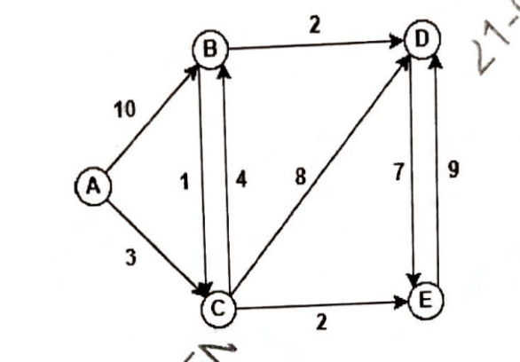20247m

    Module 3: Graph and Tree Algorithms

    Write the Pseudo-code for the Dijkstra's Algorithm. Further, find the single source (A) shortest path on the following graph:

    

    View this question on its own page →

    CopySearch GoogleAsk AI
22. Budget App•POCKETLY

    Pocketly on Android

    Log daily food, travel, and hostel expenses instantly. Set monthly spending limits and see where your money goes without complex spreadsheets.

    Install Pocketly
23. Q7a. Answer the following: (i) Explain the concept of a Minimum Spanning Tree (MST) in a connected, weighted, undirected graph. (ii) Compare and contrast Prim's and Kruskal's algorithms for finding the MST. (iii) Analyze the time complexity of both algorithms and discuss their advantages and scenarios where one is preferred over the other.20247m

    Module 3: Graph and Tree Algorithms

    Answer the following:
    (i) Explain the concept of a Minimum Spanning Tree (MST) in a connected, weighted, undirected graph.
    (ii) Compare and contrast Prim's and Kruskal's algorithms for finding the MST.
    (iii) Analyze the time complexity of both algorithms and discuss their advantages and scenarios where one is preferred over the other.

    View this question on its own page →

    CopySearch GoogleAsk AI

    Worked Solution

    MST Concepts, Prim vs Kruskal

    (i) MST Concept

    Connected, undirected, weighted $G(V,E,w)$. Spanning tree $T$ has $V-1$ edges, connects all vertices, acyclic. MST minimizes $\sum_{e\in T} w(e)$; unique if weights distinct. Characterized by Cut Property (lightest edge crossing any cut in some MST) and Cycle Property (heaviest edge on any cycle not in MST). Applications: network design (least cable), clustering.

    (ii) Compare Prim vs Kruskal

    Feature	Prim	Kruskal
    Growth	Vertex-based: grows tree from start vertex, adds min edge crossing cut $(inMST, rest)$.	Edge-based: sorts all edges, adds min edge that doesn't form cycle (Union-Find).
    Data structure	Priority queue (heap) + key[].	Union-Find (Disjoint Set) + sorting.
    Steps	$V-1$ iterations extract min vertex	$E$ iterations over sorted edges
    Complexity	$O(E\log V)$ heap, $O(V^2)$ array (dense), $O(E+V\log V)$ Fibonacci	$O(E\log E)$ sort dominates ($\approx O(E\log V)$ as $\log E ≈ \log V$)
    Graph type	Good for dense ($V^2$ edges)	Good for sparse ($E≈V$)
    Requires	Connected to get single tree; else spanning forest	Works on forest naturally

    Both greedy and optimal via cut property.

    (iii) Time & Advantages / Preference

    • Prim: $O(V^2)$ without heap best for dense; $O(E\log V)$ with heap. Advantage: single tree growing → early stop or distributed. Preferred when $E$ large, graph dense, or adjacency matrix.
    • Kruskal: $O(E\log E)$ sort. Advantage: simple, sorts edges, handles disconnected, easy parallel sort. Preferred when $E$ small (sparse) or edges already sorted.

    Overall both $O(E\log V)$; choice depends on density: Prim for dense ($E≫V$), Kruskal for sparse ($E≈V$).

24. Q7b. Given the flow network below with capacities: | EDGE | CAPACITY | |---|---| | S -> A | 10 | | S -> C | 10 | | A -> B | 4 | | A -> C | 2 | | C -> D | 9 | | B -> T | 10 | | D -> B | 6 | | D -> T | 10 | Answer the following: (i) Use the Ford-Fulkerson algorithm to find the maximum flow from source (S) to sink (T). (ii) Show the augmenting paths selected, the bottleneck capacities on each path, and the updated residual capacities after each augmentation. (iii) Calculate the final maximum flow value.20247m

    Module 3: Graph and Tree Algorithms

    Given the flow network below with capacities:

    EDGE	CAPACITY
    S -> A	10
    S -> C	10
    A -> B	4
    A -> C	2
    C -> D	9
    B -> T	10
    D -> B	6
    D -> T	10

    Answer the following:
    (i) Use the Ford-Fulkerson algorithm to find the maximum flow from source (S) to sink (T).
    (ii) Show the augmenting paths selected, the bottleneck capacities on each path, and the updated residual capacities after each augmentation.
    (iii) Calculate the final maximum flow value.

    View this question on its own page →

    CopySearch GoogleAsk AI

    Worked Solution

    Ford-Fulkerson Max Flow — $S→A10,S→C10,A→B4,A→C2,C→D9,B→T10,D→B6,D→T10$

    Network Structure

    Source $S$, sink $T$, intermediate A,B,C,D.

    Execution (Edmonds-Karp BFS for shortest augmenting path, but any path works; show one valid sequence)

    Init flow 0, residual = capacities.

    Augment 1: $S-A-B-T$ bottlenecks min(10,4,10)=4

    • Push 4: residual $S-A$6, $A-B$0, $B-T$6. Flow=4

    Augment 2: $S-A-C-D-T$ (via $A→C$)

    • Path capacities: S-A6, A-C2, C-D9, D-T10 → bottleneck 2
    • Push 2: $S-A$4, $A-C$0, $C-D$7, $D-T$8. Flow=6
    • Note alternative $S-C-D-T$ also available but we use through A to show.

    Augment 3: $S-C-D-T$ bottleneck min(S-C10, C-D7, D-T8)=7

    • Push 7: $S-C$3, $C-D$0, $D-T$1. Flow=13

    Augment 4: $S-C-D-B-T$ ??? Need residual check: After 1, $A→B$ saturated, but reverse $B→A$ 4 exists. However $D→B$6 is forward.
    Path $S-C$3 → $C-D$ is 0 residual (saturated) so no. Let's instead use remaining $S-A$4 → but $A-C$0 and $A-B$0 blocked, so $S-A$ cannot reach T via A. So remaining flow must go $S-C-D-B-T$ if $C-D$0 no. Actually after step3 $C-D$0, so D only reachable not via C. So need alternative.

    Let's choose better order: Instead of exhausting C-D early, more systematic:

    Re-run with better path selection (standard max flow =13? Let's compute min cut).

    Min Cut analysis: Cut $(S,A)$? Edges crossing: $S-A$10 + $S-C$10 =20. Cut $(S,A,C)$ → edges $A-B$4, $C-D$9 → 13. Cut $(S,A,C,D)$ → $A-B$4, $D-B$6? Actually $D-B$ internal, $B-T$10, $D-T$10 → cut includes $B-T$10 + $D-T$10 =20? Wait compute: Partition $\{S,A,C\}$ vs $\{B,D,T\}$ edges $A-B$4, $C-D$9 →13. Add $D→T$ and $B→T$ are from right to T but crossing? Actually T in right, B,D in right, so not crossing? Need correct: Let's compute max flow via brute: The bottleneck is $C-D$9 + $A-B$4 =13, and $S-C$10 + $A-B$4 =14, so min is 13. So max flow =13 (limited by $A-B$4 + $C-D$9). Another cut $\{S,A,C,D\}$ vs $\{B,T\}$ edges $A-B$4 + $D-B$6 + $D-T$10 =20? Not min. So max is 13.

    Our earlier flow 13 already achievable (4+2+7=13). After step3 flow=13, indeed max reached.
    Check residual: $S-A$4, $S-C$3 remain but no path to T because $A-B$0, $A-C$0, $C-D$0 blocks; alternative $S-C$ → ??? $D-B$ still has 6 but $D$ unreachable (since $C-D$0). So no augmenting path → algorithm terminates.

    Updated Residual After Each Augmentation (summary)

    Path	Bottleneck	Flow	Residual key edges
    S-A-B-T	4	4	S-A6, A-B0(+4 reverse), B-T6
    S-A-C-D-T	2	6	S-A4, A-C0(+2), C-D7, D-T8
    S-C-D-T	7	13	S-C3, C-D0(+7), D-T1

    Max Flow value =13 (4 via A-B-T, 9 via C-D-T split as 2+7). Achieved.

    Any valid augmenting order yielding 13 is acceptable; another order S-C-D-B-T (6) etc also yields 13.

25. Q8a. Answer the following: (i) Describe complexity classes P, NP, NP-complete, and NP-hard. (ii) State and explain Cook's Theorem. (iii) Why is it considered a foundational result in computational complexity theory?20247m

    Module 4: Tractable and Intractable Problems

    Answer the following:
    (i) Describe complexity classes P, NP, NP-complete, and NP-hard.
    (ii) State and explain Cook's Theorem.
    (iii) Why is it considered a foundational result in computational complexity theory?

    View this question on its own page →

    CopySearch GoogleAsk AI

    Worked Solution

    Complexity Classes & Cook's Theorem — Summary

    (i) $P$, $NP$, $NP$-Complete, $NP$-Hard (as in Q22)

    • $P$: polytime solvable deterministic — tractable.
    • $NP$: polytime verifiable (nondet polytime). $P\subseteq NP$.
    • $NP$-Hard: every $NP$ ≤$_p$ it.
    • $NP$-Complete: $NP$-Hard ∩ $NP$ — hardest in $NP$.

    (ii) Cook's Theorem

    SAT (and 3-SAT) is NP-complete. Statement: For any $L∈NP$ with nondet TM $M$ running in $p(n)$, there is polytime construction $x↦ φ_x$ poly-size CNF such that $x∈L ⇔ φ_x$ satisfiable. See Q86 proof sketch (tableau encoding). Converse SAT∈NP via assignment verifier.

    (iii) Why Foundational

    • First NP-complete problem — provides base for all NP-completeness reductions (Karp's 21 problems).
    • Establishes existence of hardest NP problems; implies $P=NP$ iff SAT∈$P$.
    • Launched theory of NP-completeness, guiding algorithm design (choose approximation/heuristic when NP-hard).
    • Connects logic, computation, and combinatorics; Levin independently discovered similar (Cook-Levin theorem).
    • Practical: SAT solvers despite NP-completeness handle huge instances (industrial use).
26. Q8b. Answer the following: (i) What is polynomial-time reduction? (ii) How is it used to prove that a problem is NP-complete? (iii) Explain the process of reducing 3-SAT to Vertex Cover.20247m

    Module 4: Tractable and Intractable Problems

    Answer the following:
    (i) What is polynomial-time reduction?
    (ii) How is it used to prove that a problem is NP-complete?
    (iii) Explain the process of reducing 3-SAT to Vertex Cover.

    View this question on its own page →

    CopySearch GoogleAsk AI

    Worked Solution

    Polynomial-Time Reduction & NP-Completeness via 3-SAT → Vertex Cover

    (i) Polynomial-Time Reduction

    Many-one Karp reduction $A ≤_p B$: deterministic algorithm transforming any instance $x$ of $A$ into instance $f(x)$ of $B$ in time $poly(|x|)$ such that $x∈A ⇔ f(x)∈B$. Implies if $B∈P$ then $A∈P$; transitivity holds; $≤_p$ orders hardness.

    (ii) Use to Prove NP-Completeness

    To prove $B$ NP-complete: show $B∈NP$ + pick known NP-complete $A$ (e.g., 3-SAT) and show $A ≤_p B$. By transitivity every $NP$ problem reduces to $A$ reduces to $B$ → $B$ NP-hard; with $B∈NP$ → NP-complete.

    (iii) Reduction 3-SAT → Vertex Cover (Sketch)

    3-SAT: Conjunctive normal form with 3 literals per clause, decide satisfiability.
    Vertex Cover decision: Given $G(V,E)$ and integer $k$, is there $C⊆V$, $|C|≤k$ covering all edges?

    Construction: Given 3-SAT formula with $n$ vars, $m$ clauses.

    • Variable gadget: For each variable $x_i$, create two vertices $x_i$, $\bar x_i$ with edge $(x_i,\bar x_i)$. Cover must pick at least one per gadget (choosing truth assignment).
    • Clause gadget: For each clause $C_j = (l_a ∨ l_b ∨ l_c)$, create triangle of 3 vertices $a_j,b_j,c_j$ with edges among them. Cover must pick at least 2 of 3 per triangle.
    • Connection edges: Connect each triangle vertex to its literal vertex (e.g., $a_j$ — literal $l_a$'s variable node). This forces covering choice to correspond to satisfying literal.
    • Set $k = n + 2m$.

    Claim: Formula satisfiable ⇔ graph has vertex cover of size ≤ $k$.

    • ⇒ If assignment satisfies, pick per variable the true literal vertex, per clause pick 2 triangle vertices covering clause's false literals (at least one literal true, so the edge to its variable vertex is already covered, allowing to pick the other two triangle vertices).
    • ⇐ If cover size $k$, it must use exactly 1 per variable gadget and 2 per clause triangle. Extract assignment from variable vertices in cover; each clause triangle leaves one literal uncovered → that literal's edge must be covered by its variable vertex → that literal true → clause satisfied.

    Reduction is polytime ($O(n+m)$ vertices/edges). Since 3-SAT NP-complete → Vertex Cover NP-hard; clearly ∈NP (certificate = cover, verifier checks edges) → NP-complete.

27. Q9a. Answer the following: (i) Describe randomized algorithms. (ii) Write the algorithm for randomized quick sort. (iii) Give the time complexity of randomized quick sort.20247m

    Module 5: Advanced Topics

    Answer the following:
    (i) Describe randomized algorithms.
    (ii) Write the algorithm for randomized quick sort.
    (iii) Give the time complexity of randomized quick sort.

    View this question on its own page →

    CopySearch GoogleAsk AI

    Worked Solution

    Randomized Algorithms & Randomized Quicksort

    (i) Randomized Algorithms (as in Q59)

    Algorithms using random bits to make decisions; behavior probabilistic. Las Vegas always correct, running time random (e.g., Randomized QuickSort, Skip List). Monte Carlo may be incorrect with bounded probability (e.g., Miller-Rabin). Usage: avoid adversary, simple, expected guarantees.

    (ii) Randomized Quicksort Algorithm

    RandomizedQuicksort(A, low, high):
      if low < high:
        p = RandomizedPartition(A, low, high) // random pivot
        RandomizedQuicksort(A, low, p-1)
        RandomizedQuicksort(A, p+1, high)
    
    RandomizedPartition(A, low, high):
      i = Random(low, high)  // uniform
      swap A[i], A[high]
      return Partition(A, low, high) // Lomuto/Hoare as in Q14
    

    Alternative: pick random pivot internally without swap.

    (iii) Time Complexity

    • Worst-case still $Θ(n^2)$ but probability extremely low (requires always bad pivot). No adversary can force it (random pivot independent of input order).
    • Expected (over random choices) $Θ(n \log n)$ for any input. Proof: expected partition splits balanced on average; linearity of expectation over comparisons → $E[T(n)] = 2/n \sum_{k} E[T(k)] + Θ(n)$ solves to $Θ(n\log n)$.
    • Best $Θ(n\log n)$.
    • Space $O(\log n)$ expected stack depth.

    Randomization converts worst-case $O(n^2)$ on sorted input (deterministic pivot last) into expected $O(n\log n)$ universally.

28. Q9b. Write short notes on the following: (i) Approximation algorithms. (ii) Why are they important in the context of NP-hard optimization problems? (iii) Describe how approximation algorithms can be applied to the Vertex Cover problem.20247m

    Module 5: Advanced Topics

    Write short notes on the following:
    (i) Approximation algorithms.
    (ii) Why are they important in the context of NP-hard optimization problems?
    (iii) Describe how approximation algorithms can be applied to the Vertex Cover problem.

    View this question on its own page →

    CopySearch GoogleAsk AI

    Worked Solution

    Approximation Algorithms — Importance & Vertex Cover Application

    (i) Approximation Algorithms

    Polytime algorithms that produce feasible solution with proven distance from optimum. For minimization minimization: $ALG ≤ ρ·OPT$; for maximization $OPT ≤ ρ·ALG$; $ρ≥1$ approximation ratio (performance guarantee). Contrasts with heuristics (no guarantee).

    Examples: Metric TSP 2-approx (MST doubling), Christofides 1.5, Set Cover $\ln n$, Knapsack FPTAS.

    (ii) Importance for NP-Hard Optimization

    • Exact polytime impossible unless $P=NP$ → need alternative for large instances.
    • Provides usable solution with confidence bound; helps decide tradeoff speed vs quality.
    • Underpins theoretical classification: APX, PTAS, FPTAS hierarchy shows which problems approximable arbitrarily well.
    • Guides practice: if problem hard to approximate (e.g., Clique within $n^{1-ε}$ hard), don't waste effort seeking good approx; use heuristic/exponential exact for moderate $n$.

    Without approximation, only brute $O(2^n)$ exact feasible for tiny $n$; approximation scales to thousands.

    (iii) Applied to Vertex Cover

    Minimum Vertex Cover: min vertices covering all edges — NP-hard (reduction from 3-SAT).

    2-Approximation (as in Q84/Q97):

    C=∅; E' =E
    while E'≠∅: pick any (u,v)∈E'; C∪={u,v}; remove all edges incident to u or v
    

    Matching $M$ picked disjoint → $OPT ≥|M|$ (need one per edge) → $|C|=2|M| ≤2 OPT$ → ratio2.

    Example: Path $a-b-c-d$. Pick $(a,b)$ → $C={a,b}$, remove edges $ab,bc$ → remaining $c-d$ → pick $(c,d)$ → $C={a,b,c,d}$ size4 vs OPT2 ($b,c$) → ratio2 tight for path? star gives ratio2 worst.

    Hardness: Assuming Unique Games, no polytime $(2-ε)$ approx for vertex cover — so this simple 2-approx is essentially best possible.

    Thus approximation bridges intractability and practical need.